| | |  GitHub पर स्रोत देखें GitHub पर स्रोत देखें | |
यह ली एट अल द्वारा नामित 16 मार्च 2020 पेपर का एक TensorFlow प्रायिकता पोर्ट है। हम आधुनिक महामारी विज्ञान मॉडलिंग की सेटिंग में TFP की कुछ क्षमताओं को प्रदर्शित करते हुए, TensorFlow Probability प्लेटफॉर्म पर मूल लेखकों के तरीकों और परिणामों को ईमानदारी से पुन: पेश करते हैं। TensorFlow पर पोर्ट करने से हमें मूल मैटलैब कोड की तुलना में ~10x स्पीडअप मिलता है, और चूंकि TensorFlow Probability व्यापक रूप से वेक्टरकृत बैच गणना का समर्थन करता है, इसलिए सैकड़ों स्वतंत्र प्रतिकृतियों के लिए अनुकूल रूप से स्केल करता है।
मूल पेपर
रुइयुन ली, सेन पेई, बिन चेन, यिमेंग सॉन्ग, ताओ झांग, वान यांग और जेफरी शमन। पर्याप्त अनिर्दिष्ट संक्रमण उपन्यास कोरोनवायरस (SARS-CoV2) के तेजी से प्रसार की सुविधा प्रदान करता है। (2020), डोई: https://doi.org/10.1126/science.abb3221 ।
सार:। "प्रसार और गैर-दस्तावेजी उपन्यास कोरोना (सार्स-CoV2) संक्रमण के contagiousness का आकलन समग्र प्रसार और इस रोग की महामारी संभावित को समझने के लिए महत्वपूर्ण है यहाँ हम गतिशीलता डेटा, एक साथ संयोजन के रूप में चीन के भीतर सूचित संक्रमण की टिप्पणियों का उपयोग करें, गैर-दस्तावेजी संक्रमणों के अंश और उनकी संक्रामकता सहित SARS-CoV2 से जुड़ी महत्वपूर्ण महामारी विज्ञान विशेषताओं का पता लगाने के लिए नेटवर्क गतिशील मेटापॉपुलेशन मॉडल और बायेसियन अनुमान। हमारा अनुमान है कि सभी संक्रमणों में से 86% अनिर्दिष्ट थे (95% सीआई: [82%-90%] ) 23 जनवरी 2020 से पहले यात्रा प्रतिबंध। प्रति व्यक्ति, अनिर्दिष्ट संक्रमणों की संचरण दर प्रलेखित संक्रमणों का 55% थी ([46% –62%]), फिर भी, उनकी अधिक संख्या के कारण, गैर-दस्तावेज संक्रमण 79 के लिए संक्रमण का स्रोत थे। प्रलेखित मामलों का%। ये निष्कर्ष SARS-CoV2 के तेजी से भौगोलिक प्रसार की व्याख्या करते हैं और संकेत करते हैं कि इस वायरस की रोकथाम विशेष रूप से चुनौतीपूर्ण होगी।"
Github लिंक कोड और डेटा के लिए।
अवलोकन
मॉडल एक है पूरक रोग मॉडल के लिए "अतिसंवेदनशील", "उजागर" (संक्रमित लेकिन अभी तक संक्रामक नहीं), "संक्रामक कभी नहीं से प्रलेखित", और "अंत में प्रलेखित संक्रामक" डिब्बों के साथ,। दो उल्लेखनीय विशेषताएं हैं: 375 चीनी शहरों में से प्रत्येक के लिए अलग-अलग डिब्बे, इस धारणा के साथ कि लोग एक शहर से दूसरे शहर में कैसे यात्रा करते हैं; और संक्रमण की जानकारी देने में देरी, ताकि एक मामला है कि हो जाता है "अंत में प्रलेखित संक्रामक" दिन पर \(t\) एक स्टोकेस्टिक बाद में दिन तक मनाया मामले में गिना जाता है में दिखाई नहीं देता।
मॉडल मानता है कि कभी भी प्रलेखित मामले मामूली होने के कारण अनिर्दिष्ट हो जाते हैं, और इस प्रकार दूसरों को कम दर पर संक्रमित करते हैं। मूल पेपर में रुचि का मुख्य पैरामीटर उन मामलों का अनुपात है जो अनिर्दिष्ट हो जाते हैं, मौजूदा संक्रमण की सीमा और बीमारी के प्रसार पर अनिर्दिष्ट संचरण के प्रभाव का अनुमान लगाने के लिए।
यह कोलाब बॉटम-अप स्टाइल में कोड वॉकथ्रू के रूप में संरचित है। क्रम में, हम करेंगे
- डेटा को निगलना और संक्षेप में जांचना,
- राज्य स्थान और मॉडल की गतिशीलता को परिभाषित करें,
- ली एट अल, और . के बाद मॉडल में अनुमान लगाने के लिए कार्यों का एक सूट बनाएं
- उन्हें आमंत्रित करें और परिणामों की जांच करें। स्पोइलर: वे कागज के समान ही निकलते हैं।
स्थापना और पायथन आयात
pip3 install -q tf-nightly tfp-nightly
import collections
import io
import requests
import time
import zipfile

import matplotlib.pyplot as plt
import numpy as np
import pandas as pd

import tensorflow.compat.v2 as tf
import tensorflow_probability as tfp
from tensorflow_probability.python.internal import samplers

tfd = tfp.distributions
tfes = tfp.experimental.sequential
डेटा आयात
आइए डेटा को जीथब से आयात करें और उसमें से कुछ का निरीक्षण करें।
r = requests.get('https://raw.githubusercontent.com/SenPei-CU/COVID-19/master/Data.zip')
z = zipfile.ZipFile(io.BytesIO(r.content))
z.extractall('/tmp/')
raw_incidence = pd.read_csv('/tmp/data/Incidence.csv')
raw_mobility = pd.read_csv('/tmp/data/Mobility.csv')
raw_population = pd.read_csv('/tmp/data/pop.csv')
नीचे हम प्रति दिन कच्ची घटनाओं की संख्या देख सकते हैं। हम पहले 14 दिनों (10 जनवरी से 23 जनवरी) में सबसे अधिक रुचि रखते हैं, क्योंकि यात्रा प्रतिबंध 23 तारीख को लगाए गए थे। पेपर 10-23 जनवरी और 23 जनवरी+ को अलग-अलग मापदंडों के साथ मॉडलिंग करके इससे निपटता है; हम अपने प्रजनन को पहले की अवधि तक ही सीमित रखेंगे।
raw_incidence.drop('Date', axis=1)  # The 'Date' column is all 1/18/21
# Luckily the days are in order, starting on January 10th, 2020.
आइए वुहान की घटनाओं की गिनती की विवेक-जांच करें।
plt.plot(raw_incidence.Wuhan, '.-')
plt.title('Wuhan incidence counts over 1/10/20 - 02/08/20')
plt.show()
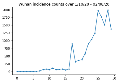
अब तक सब ठीक है। अब प्रारंभिक जनसंख्या मायने रखती है।
raw_population
आइए यह भी देखें और रिकॉर्ड करें कि कौन सी एंट्री वुहान की है।
raw_population['City'][169]
'Wuhan'
WUHAN_IDX = 169
और यहां हम विभिन्न शहरों के बीच गतिशीलता मैट्रिक्स देखते हैं। यह पहले 14 दिनों में विभिन्न शहरों के बीच आने-जाने वाले लोगों की संख्या के लिए एक प्रॉक्सी है। यह 2018 चंद्र नव वर्ष के मौसम के लिए Tencent द्वारा प्रदान किए गए GPS रिकॉर्ड से प्राप्त हुआ है। किसी अज्ञात (अनुमान के अधीन) निरंतर कारक 2020 के मौसम के दौरान ली एट अल मॉडल गतिशीलता \(\theta\) बार इस।
raw_mobility
अंत में, आइए इन सभी को numpy arrays में प्रीप्रोसेस करें जिनका हम उपभोग कर सकते हैं।
# The given populations are only "initial" because of intercity mobility during
# the holiday season.
initial_population = raw_population['Population'].to_numpy().astype(np.float32)
गतिशीलता डेटा को [एल, एल, टी]-आकार वाले टेंसर में कनवर्ट करें, जहां एल स्थानों की संख्या है, और टी टाइमस्टेप्स की संख्या है।
daily_mobility_matrices = []
for i in range(1, 15):
  day_mobility = raw_mobility[raw_mobility['Day'] == i]

  # Make a matrix of daily mobilities.
  z = pd.crosstab(
      day_mobility.Origin,
      day_mobility.Destination,
      values=day_mobility['Mobility Index'], aggfunc='sum', dropna=False)

  # Include every city, even if there are no rows for some in the raw data on
  # some day.  This uses the sort order of `raw_population`.
  z = z.reindex(index=raw_population['City'], columns=raw_population['City'],
                fill_value=0)
  # Finally, fill any missing entries with 0. This means no mobility.
  z = z.fillna(0)
  daily_mobility_matrices.append(z.to_numpy())

mobility_matrix_over_time = np.stack(daily_mobility_matrices, axis=-1).astype(
    np.float32)
अंत में देखे गए संक्रमणों को लें और एक [एल, टी] तालिका बनाएं।
# Remove the date parameter and take the first 14 days.
observed_daily_infectious_count = raw_incidence.to_numpy()[:14, 1:]
observed_daily_infectious_count = np.transpose(
    observed_daily_infectious_count).astype(np.float32)
और दोबारा जांच लें कि हमें अपनी इच्छानुसार आकार मिले हैं। एक अनुस्मारक के रूप में, हम 375 शहरों और 14 दिनों के साथ काम कर रहे हैं।
print('Mobility Matrix over time should have shape (375, 375, 14): {}'.format(
    mobility_matrix_over_time.shape))
print('Observed Infectious should have shape (375, 14): {}'.format(
    observed_daily_infectious_count.shape))
print('Initial population should have shape (375): {}'.format(
    initial_population.shape))
Mobility Matrix over time should have shape (375, 375, 14): (375, 375, 14)
Observed Infectious should have shape (375, 14): (375, 14)
Initial population should have shape (375): (375,)
राज्य और पैरामीटर्स को परिभाषित करना
आइए अपने मॉडल को परिभाषित करना शुरू करें। मॉडल हम प्रजनन कर रहे हैं एक का एक प्रकार है सेईर मॉडल । इस मामले में हमारे पास निम्नलिखित समय-भिन्न राज्य हैं:
- \(S\): प्रत्येक शहर में बीमारी के लिए अतिसंवेदनशील लोगों की संख्या।
- \(E\): रोग के संपर्क में प्रत्येक शहर में लोगों की संख्या लेकिन संक्रामक नहीं अभी तक। जैविक रूप से, यह बीमारी के अनुबंध से मेल खाती है, जिसमें सभी उजागर लोग अंततः संक्रामक हो जाते हैं।
- \(I^u\): प्रत्येक शहर जो संक्रामक लेकिन undocumented हैं में लोगों की संख्या। मॉडल में, इसका वास्तव में अर्थ है "कभी भी प्रलेखित नहीं किया जाएगा"।
- \(I^r\): प्रत्येक शहर जो संक्रामक है और इस तरह के रूप में दस्तावेज हैं में लोगों की संख्या। ली एट अल मॉडल रिपोर्टिंग विलंब, तो \(I^r\) वास्तव में की तरह कुछ से मेल खाती है "मामले काफी गंभीर भविष्य में कुछ बिंदु पर प्रलेखित किया जाना है।"
जैसा कि हम नीचे देखेंगे, हम समय पर एक एन्सेम्बल-समायोजित कलमन फ़िल्टर (EAKF) चलाकर इन राज्यों का अनुमान लगाएंगे। ईएकेएफ का राज्य वेक्टर इनमें से प्रत्येक मात्रा के लिए एक शहर-अनुक्रमित वेक्टर है।
मॉडल में निम्नलिखित अचूक वैश्विक, समय-अपरिवर्तनीय पैरामीटर हैं:
- \(\beta\): दस्तावेज संक्रामक व्यक्तियों की वजह से संचरण दर।
- \(\mu\): गैर-दस्तावेजी संक्रामक व्यक्तियों की वजह से रिश्तेदार संचरण दर। यह उत्पाद के माध्यम से कार्य करेगा \(\mu \beta\)।
- \(\theta\): इंटरसिटी गतिशीलता कारक। यह गतिशीलता डेटा की कम रिपोर्टिंग (और 2018 से 2020 तक जनसंख्या वृद्धि के लिए) के लिए एक सुधार कारक से अधिक है।
- \(Z\): औसत ऊष्मायन अवधि (यानी, "उजागर" राज्य में समय)।
- \(\alpha\)(अंततः) दस्तावेज यह संक्रमण काफी गंभीर होने के लिए के अंश है:।
- \(D\): संक्रमण की औसत अवधि (यानी, या तो "संक्रामक" राज्य में समय)।
हम राज्यों के लिए EAKF के चारों ओर एक पुनरावृत्त-फ़िल्टरिंग लूप के साथ इन मापदंडों के लिए बिंदु अनुमानों का अनुमान लगाएंगे।
मॉडल गैर-अनुमानित स्थिरांक पर भी निर्भर करता है:
- \(M\): इंटरसिटी गतिशीलता मैट्रिक्स। यह समय-भिन्न है और माना जाता है। याद रखें कि यह निष्कर्ष निकाला पैरामीटर द्वारा बढ़ाया है \(\theta\) शहरों के बीच वास्तविक जनसंख्या आंदोलनों देने के लिए।
- \(N\): प्रत्येक शहर में लोगों की कुल संख्या। प्रारंभिक आबादी लिया जाता है के रूप में दिया, और जनसंख्या के समय भिन्नता गतिशीलता संख्या से गणना की जाती है \(\theta M\)।
सबसे पहले, हम अपने राज्यों और मापदंडों को रखने के लिए खुद को कुछ डेटा संरचनाएं देते हैं।
SEIRComponents = collections.namedtuple(
  typename='SEIRComponents',
  field_names=[
    'susceptible',              # S
    'exposed',                  # E
    'documented_infectious',    # I^r
    'undocumented_infectious',  # I^u
    # This is the count of new cases in the "documented infectious" compartment.
    # We need this because we will introduce a reporting delay, between a person
    # entering I^r and showing up in the observable case count data.
    # This can't be computed from the cumulative `documented_infectious` count,
    # because some portion of that population will move to the 'recovered'
    # state, which we aren't tracking explicitly.
    'daily_new_documented_infectious'])

ModelParams = collections.namedtuple(
    typename='ModelParams',
    field_names=[
      'documented_infectious_tx_rate',             # Beta
      'undocumented_infectious_tx_relative_rate',  # Mu
      'intercity_underreporting_factor',           # Theta
      'average_latency_period',                    # Z
      'fraction_of_documented_infections',         # Alpha
      'average_infection_duration'                 # D
    ]
)
हम मापदंडों के मूल्यों के लिए ली एट अल की सीमा को भी कोड करते हैं।
PARAMETER_LOWER_BOUNDS = ModelParams(
    documented_infectious_tx_rate=0.8,
    undocumented_infectious_tx_relative_rate=0.2,
    intercity_underreporting_factor=1.,
    average_latency_period=2.,
    fraction_of_documented_infections=0.02,
    average_infection_duration=2.
)

PARAMETER_UPPER_BOUNDS = ModelParams(
    documented_infectious_tx_rate=1.5,
    undocumented_infectious_tx_relative_rate=1.,
    intercity_underreporting_factor=1.75,
    average_latency_period=5.,
    fraction_of_documented_infections=1.,
    average_infection_duration=5.
)
SEIR गतिशीलता
यहां हम मापदंडों और राज्य के बीच संबंध को परिभाषित करते हैं।
ली एट अल (पूरक सामग्री, eqns 1-5) से समय-गतिकी समीकरण इस प्रकार हैं:
\(\frac{dS_i}{dt} = -\beta \frac{S_i I_i^r}{N_i} - \mu \beta \frac{S_i I_i^u}{N_i} + \theta \sum_k \frac{M_{ij} S_j}{N_j - I_j^r} - + \theta \sum_k \frac{M_{ji} S_j}{N_i - I_i^r}\)
\(\frac{dE_i}{dt} = \beta \frac{S_i I_i^r}{N_i} + \mu \beta \frac{S_i I_i^u}{N_i} -\frac{E_i}{Z} + \theta \sum_k \frac{M_{ij} E_j}{N_j - I_j^r} - + \theta \sum_k \frac{M_{ji} E_j}{N_i - I_i^r}\)
\(\frac{dI^r_i}{dt} = \alpha \frac{E_i}{Z} - \frac{I_i^r}{D}\)
\(\frac{dI^u_i}{dt} = (1 - \alpha) \frac{E_i}{Z} - \frac{I_i^u}{D} + \theta \sum_k \frac{M_{ij} I_j^u}{N_j - I_j^r} - + \theta \sum_k \frac{M_{ji} I^u_j}{N_i - I_i^r}\)
\(N_i = N_i + \theta \sum_j M_{ij} - \theta \sum_j M_{ji}\)
आपको याद दिला दें, जैसा कि \(i\) और \(j\) सबस्क्रिप्ट सूचकांक शहरों। ये समीकरण के माध्यम से रोग के समय-विकास को दर्शाते हैं
- संक्रामक व्यक्तियों के संपर्क में आने से अधिक संक्रमण हो सकता है;
- "उजागर" से "संक्रामक" राज्यों में से एक में रोग की प्रगति;
- रोग की प्रगति "संक्रामक" अवस्था से ठीक होने की ओर होती है, जिसे हम प्रतिरूपित जनसंख्या से हटाकर मॉडल बनाते हैं;
- उजागर या गैर-दस्तावेज-संक्रामक व्यक्तियों सहित अंतर-शहर गतिशीलता; तथा
- अंतर-शहर गतिशीलता के माध्यम से दैनिक शहर की आबादी का समय-भिन्नता।
ली एट अल के बाद, हम मानते हैं कि गंभीर मामलों वाले लोग अंततः रिपोर्ट किए जाने के लिए शहरों के बीच यात्रा नहीं करते हैं।
इसके अलावा ली एट अल का पालन करते हुए, हम इन गतिकी को शब्द-वार पॉइसन शोर के अधीन मानते हैं, अर्थात, प्रत्येक शब्द वास्तव में एक पॉइसन की दर है, एक नमूना जिसमें से सही परिवर्तन होता है। पॉइसन शोर शब्द-वार है क्योंकि घटाना (जोड़ने के विपरीत) पॉसों के नमूने पॉइसन-वितरित परिणाम नहीं देते हैं।
हम क्लासिक चौथे क्रम के रनगे-कुट्टा इंटीग्रेटर के साथ इन गतिशीलता को समय पर आगे बढ़ाएंगे, लेकिन पहले आइए उस फ़ंक्शन को परिभाषित करें जो उनकी गणना करता है (पॉइसन शोर के नमूने सहित)।
def sample_state_deltas(
    state, population, mobility_matrix, params, seed, is_deterministic=False):
  """Computes one-step change in state, including Poisson sampling.

  Note that this is coded to support vectorized evaluation on arbitrary-shape
  batches of states.  This is useful, for example, for running multiple
  independent replicas of this model to compute credible intervals for the
  parameters.  We refer to the arbitrary batch shape with the conventional
  `B` in the parameter documentation below.  This function also, of course,
  supports broadcasting over the batch shape.

  Args:
    state: A `SEIRComponents` tuple with fields Tensors of shape
      B + [num_locations] giving the current disease state.
    population: A Tensor of shape B + [num_locations] giving the current city
      populations.
    mobility_matrix: A Tensor of shape B + [num_locations, num_locations] giving
      the current baseline inter-city mobility.
    params: A `ModelParams` tuple with fields Tensors of shape B giving the
      global parameters for the current EAKF run.
    seed: Initial entropy for pseudo-random number generation.  The Poisson
      sampling is repeatable by supplying the same seed.
    is_deterministic: A `bool` flag to turn off Poisson sampling if desired.

  Returns:
    delta: A `SEIRComponents` tuple with fields Tensors of shape
      B + [num_locations] giving the one-day changes in the state, according
      to equations 1-4 above (including Poisson noise per Li et al).
  """
  undocumented_infectious_fraction = state.undocumented_infectious / population
  documented_infectious_fraction = state.documented_infectious / population

  # Anyone not documented as infectious is considered mobile
  mobile_population = (population - state.documented_infectious)
  def compute_outflow(compartment_population):
    raw_mobility = tf.linalg.matvec(
        mobility_matrix, compartment_population / mobile_population)
    return params.intercity_underreporting_factor * raw_mobility
  def compute_inflow(compartment_population):
    raw_mobility = tf.linalg.matmul(
        mobility_matrix,
        (compartment_population / mobile_population)[..., tf.newaxis],
        transpose_a=True)
    return params.intercity_underreporting_factor * tf.squeeze(
        raw_mobility, axis=-1)

  # Helper for sampling the Poisson-variate terms.
  seeds = samplers.split_seed(seed, n=11)
  if is_deterministic:
    def sample_poisson(rate):
      return rate
  else:
    def sample_poisson(rate):
      return tfd.Poisson(rate=rate).sample(seed=seeds.pop())

  # Below are the various terms called U1-U12 in the paper. We combined the
  # first two, which should be fine; both are poisson so their sum is too, and
  # there's no risk (as there could be in other terms) of going negative.
  susceptible_becoming_exposed = sample_poisson(
      state.susceptible *
      (params.documented_infectious_tx_rate *
       documented_infectious_fraction +
       (params.undocumented_infectious_tx_relative_rate *
        params.documented_infectious_tx_rate) *
       undocumented_infectious_fraction))  # U1 + U2

  susceptible_population_inflow = sample_poisson(
      compute_inflow(state.susceptible))  # U3
  susceptible_population_outflow = sample_poisson(
      compute_outflow(state.susceptible))  # U4

  exposed_becoming_documented_infectious = sample_poisson(
      params.fraction_of_documented_infections *
      state.exposed / params.average_latency_period)  # U5
  exposed_becoming_undocumented_infectious = sample_poisson(
      (1 - params.fraction_of_documented_infections) *
      state.exposed / params.average_latency_period)  # U6

  exposed_population_inflow = sample_poisson(
      compute_inflow(state.exposed))  # U7
  exposed_population_outflow = sample_poisson(
      compute_outflow(state.exposed))  # U8

  documented_infectious_becoming_recovered = sample_poisson(
      state.documented_infectious /
      params.average_infection_duration)  # U9
  undocumented_infectious_becoming_recovered = sample_poisson(
      state.undocumented_infectious /
      params.average_infection_duration)  # U10

  undocumented_infectious_population_inflow = sample_poisson(
      compute_inflow(state.undocumented_infectious))  # U11
  undocumented_infectious_population_outflow = sample_poisson(
      compute_outflow(state.undocumented_infectious))  # U12

  # The final state_deltas
  return SEIRComponents(
      # Equation [1]
      susceptible=(-susceptible_becoming_exposed +
                   susceptible_population_inflow +
                   -susceptible_population_outflow),
      # Equation [2]
      exposed=(susceptible_becoming_exposed +
               -exposed_becoming_documented_infectious +
               -exposed_becoming_undocumented_infectious +
               exposed_population_inflow +
               -exposed_population_outflow),
      # Equation [3]
      documented_infectious=(
          exposed_becoming_documented_infectious +
          -documented_infectious_becoming_recovered),
      # Equation [4]
      undocumented_infectious=(
          exposed_becoming_undocumented_infectious +
          -undocumented_infectious_becoming_recovered +
          undocumented_infectious_population_inflow +
          -undocumented_infectious_population_outflow),
      # New to-be-documented infectious cases, subject to the delayed
      # observation model.
      daily_new_documented_infectious=exposed_becoming_documented_infectious)
यहाँ इंटीग्रेटर है। यह करने के लिए के माध्यम से PRNG बीज गुजर के अलावा पूरी तरह मानक है, sample_state_deltas कि के लिए Runge-Kutta विधि कॉल आंशिक चरणों में से प्रत्येक में स्वतंत्र प्वासों शोर पाने के लिए कार्य करते हैं।
@tf.function(autograph=False)
def rk4_one_step(state, population, mobility_matrix, params, seed):
  """Implement one step of RK4, wrapped around a call to sample_state_deltas."""
  # One seed for each RK sub-step
  seeds = samplers.split_seed(seed, n=4)

  deltas = tf.nest.map_structure(tf.zeros_like, state)
  combined_deltas = tf.nest.map_structure(tf.zeros_like, state)

  for a, b in zip([1., 2, 2, 1.], [6., 3., 3., 6.]):
    next_input = tf.nest.map_structure(
        lambda x, delta, a=a: x + delta / a, state, deltas)
    deltas = sample_state_deltas(
        next_input,
        population,
        mobility_matrix,
        params,
        seed=seeds.pop(), is_deterministic=False)
    combined_deltas = tf.nest.map_structure(
        lambda x, delta, b=b: x + delta / b, combined_deltas, deltas)

  return tf.nest.map_structure(
      lambda s, delta: s + tf.round(delta),
      state, combined_deltas)
प्रारंभ
यहां हम कागज से आरंभीकरण योजना लागू करते हैं।
ली एट अल के बाद, हमारी अनुमान योजना एक पुनरावृत्त फ़िल्टरिंग बाहरी लूप (आईएफ-ईएकेएफ) से घिरा हुआ एक पहनावा समायोजन कलमन फ़िल्टर आंतरिक लूप होगा। कम्प्यूटेशनल रूप से, इसका मतलब है कि हमें तीन प्रकार के आरंभीकरण की आवश्यकता है:
- आंतरिक EAKF . के लिए प्रारंभिक अवस्था
- बाहरी IF के लिए प्रारंभिक पैरामीटर, जो पहले EAKF के लिए प्रारंभिक पैरामीटर भी हैं
- एक IF पुनरावृत्ति से दूसरे में पैरामीटर अपडेट करना, जो पहले के अलावा प्रत्येक EAKF के लिए प्रारंभिक पैरामीटर के रूप में कार्य करता है।
def initialize_state(num_particles, num_batches, seed):
  """Initialize the state for a batch of EAKF runs.

  Args:
    num_particles: `int` giving the number of particles for the EAKF.
    num_batches: `int` giving the number of independent EAKF runs to
      initialize in a vectorized batch.
    seed: PRNG entropy.

  Returns:
    state: A `SEIRComponents` tuple with Tensors of shape [num_particles,
      num_batches, num_cities] giving the initial conditions in each
      city, in each filter particle, in each batch member.
  """
  num_cities = mobility_matrix_over_time.shape[-2]
  state_shape = [num_particles, num_batches, num_cities]
  susceptible = initial_population * np.ones(state_shape, dtype=np.float32)
  documented_infectious = np.zeros(state_shape, dtype=np.float32)
  daily_new_documented_infectious = np.zeros(state_shape, dtype=np.float32)

  # Following Li et al, initialize Wuhan with up to 2000 people exposed
  # and another up to 2000 undocumented infectious.
  rng = np.random.RandomState(seed[0] % (2**31 - 1))
  wuhan_exposed = rng.randint(
      0, 2001, [num_particles, num_batches]).astype(np.float32)
  wuhan_undocumented_infectious = rng.randint(
      0, 2001, [num_particles, num_batches]).astype(np.float32)

  # Also following Li et al, initialize cities adjacent to Wuhan with three
  # days' worth of additional exposed and undocumented-infectious cases,
  # as they may have traveled there before the beginning of the modeling
  # period.
  exposed = 3 * mobility_matrix_over_time[
      WUHAN_IDX, :, 0] * wuhan_exposed[
          ..., np.newaxis] / initial_population[WUHAN_IDX]
  undocumented_infectious = 3 * mobility_matrix_over_time[
      WUHAN_IDX, :, 0] * wuhan_undocumented_infectious[
          ..., np.newaxis] / initial_population[WUHAN_IDX]

  exposed[..., WUHAN_IDX] = wuhan_exposed
  undocumented_infectious[..., WUHAN_IDX] = wuhan_undocumented_infectious

  # Following Li et al, we do not remove the inital exposed and infectious
  # persons from the susceptible population.
  return SEIRComponents(
      susceptible=tf.constant(susceptible),
      exposed=tf.constant(exposed),
      documented_infectious=tf.constant(documented_infectious),
      undocumented_infectious=tf.constant(undocumented_infectious),
      daily_new_documented_infectious=tf.constant(daily_new_documented_infectious))

def initialize_params(num_particles, num_batches, seed):
  """Initialize the global parameters for the entire inference run.

  Args:
    num_particles: `int` giving the number of particles for the EAKF.
    num_batches: `int` giving the number of independent EAKF runs to
      initialize in a vectorized batch.
    seed: PRNG entropy.

  Returns:
    params: A `ModelParams` tuple with fields Tensors of shape
      [num_particles, num_batches] giving the global parameters
      to use for the first batch of EAKF runs.
  """
  # We have 6 parameters. We'll initialize with a Sobol sequence,
  # covering the hyper-rectangle defined by our parameter limits.
  halton_sequence = tfp.mcmc.sample_halton_sequence(
      dim=6, num_results=num_particles * num_batches, seed=seed)
  halton_sequence = tf.reshape(
      halton_sequence, [num_particles, num_batches, 6])
  halton_sequences = tf.nest.pack_sequence_as(
      PARAMETER_LOWER_BOUNDS, tf.split(
          halton_sequence, num_or_size_splits=6, axis=-1))
  def interpolate(minval, maxval, h):
    return (maxval - minval) * h + minval
  return tf.nest.map_structure(
      interpolate,
      PARAMETER_LOWER_BOUNDS, PARAMETER_UPPER_BOUNDS, halton_sequences)

def update_params(num_particles, num_batches,
                  prev_params, parameter_variance, seed):
  """Update the global parameters between EAKF runs.

  Args:
    num_particles: `int` giving the number of particles for the EAKF.
    num_batches: `int` giving the number of independent EAKF runs to
      initialize in a vectorized batch.
    prev_params: A `ModelParams` tuple of the parameters used for the previous
      EAKF run.
    parameter_variance: A `ModelParams` tuple specifying how much to drift
      each parameter.
    seed: PRNG entropy.

  Returns:
    params: A `ModelParams` tuple with fields Tensors of shape
      [num_particles, num_batches] giving the global parameters
      to use for the next batch of EAKF runs.
  """
  # Initialize near the previous set of parameters. This is the first step
  # in Iterated Filtering.
  seeds = tf.nest.pack_sequence_as(
      prev_params, samplers.split_seed(seed, n=len(prev_params)))
  return tf.nest.map_structure(
      lambda x, v, seed: x + tf.math.sqrt(v) * tf.random.stateless_normal([
          num_particles, num_batches, 1], seed=seed),
      prev_params, parameter_variance, seeds)
देरी
इस मॉडल की महत्वपूर्ण विशेषताओं में से एक इस तथ्य का स्पष्ट रूप से ध्यान रखना है कि संक्रमण शुरू होने की तुलना में बाद में रिपोर्ट किया जाता है। यही कारण है, हम उम्मीद करते हैं कि एक व्यक्ति जो साथ लेकर चलता \(E\) के डिब्बे \(I^r\) दिन पर डिब्बे \(t\) नहीं कुछ बाद में दिन तक नमूदार रिपोर्ट मामले में गिना जाता है में दिखाई दे सकते।
हम मानते हैं कि देरी गामा-वितरित है। ली एट अल के बाद, हम आकार के लिए 1.85 का उपयोग करते हैं, और 9 दिनों की औसत रिपोर्टिंग देरी उत्पन्न करने के लिए दर को मापते हैं।
def raw_reporting_delay_distribution(gamma_shape=1.85, reporting_delay=9.):
  return tfp.distributions.Gamma(
      concentration=gamma_shape, rate=gamma_shape / reporting_delay)
हमारे अवलोकन असतत हैं, इसलिए हम कच्चे (निरंतर) देरी को निकटतम दिन तक पूरा करेंगे। हमारे पास एक सीमित डेटा क्षितिज भी है, इसलिए किसी एक व्यक्ति के लिए विलंब वितरण शेष दिनों में एक स्पष्ट है। इसलिए हम नमूने अधिक कुशलता से प्रति-शहर की भविष्यवाणी की टिप्पणियों की गणना कर सकता \(O(I^r)\) बजाय gammas, पूर्व कंप्यूटिंग बहुपद देरी संभावनाओं से।
def reporting_delay_probs(num_timesteps, gamma_shape=1.85, reporting_delay=9.):
  gamma_dist = raw_reporting_delay_distribution(gamma_shape, reporting_delay)
  multinomial_probs = [gamma_dist.cdf(1.)]
  for k in range(2, num_timesteps + 1):
    multinomial_probs.append(gamma_dist.cdf(k) - gamma_dist.cdf(k - 1))
  # For samples that are larger than T.
  multinomial_probs.append(gamma_dist.survival_function(num_timesteps))
  multinomial_probs = tf.stack(multinomial_probs)
  return multinomial_probs
इन देरी को वास्तव में नए दैनिक प्रलेखित संक्रामक गणनाओं पर लागू करने के लिए कोड यहां दिया गया है:
def delay_reporting(
    daily_new_documented_infectious, num_timesteps, t, multinomial_probs, seed):
  # This is the distribution of observed infectious counts from the current
  # timestep.

  raw_delays = tfd.Multinomial(
      total_count=daily_new_documented_infectious,
      probs=multinomial_probs).sample(seed=seed)

  # The last bucket is used for samples that are out of range of T + 1. Thus
  # they are not going to be observable in this model.
  clipped_delays = raw_delays[..., :-1]

  # We can also remove counts that are such that t + i >= T.
  clipped_delays = clipped_delays[..., :num_timesteps - t]
  # We finally shift everything by t. That means prepending with zeros.
  return tf.concat([
      tf.zeros(
          tf.concat([
              tf.shape(clipped_delays)[:-1], [t]], axis=0),
          dtype=clipped_delays.dtype),
      clipped_delays], axis=-1)
अनुमान
पहले हम अनुमान के लिए कुछ डेटा संरचनाओं को परिभाषित करेंगे।
विशेष रूप से, हम Iterated Filtering करना चाहेंगे, जो अनुमान करते समय राज्य और मापदंडों को एक साथ पैकेज करता है। तो हम एक को परिभाषित करेंगे ParameterStatePair वस्तु।
हम मॉडल में किसी भी पक्ष की जानकारी को भी पैकेज करना चाहते हैं।
ParameterStatePair = collections.namedtuple(
    'ParameterStatePair', ['state', 'params'])

# Info that is tracked and mutated but should not have inference performed over.
SideInfo = collections.namedtuple(
    'SideInfo', [
        # Observations at every time step.
        'observations_over_time',
        'initial_population',
        'mobility_matrix_over_time',
        'population',
        # Used for variance of measured observations.
        'actual_reported_cases',
        # Pre-computed buckets for the multinomial distribution.
        'multinomial_probs',
        'seed',
    ])

# Cities can not fall below this fraction of people
MINIMUM_CITY_FRACTION = 0.6

# How much to inflate the covariance by.
INFLATION_FACTOR = 1.1

INFLATE_FN = tfes.inflate_by_scaled_identity_fn(INFLATION_FACTOR)
यहां संपूर्ण अवलोकन मॉडल है, जिसे एन्सेम्बल कलमैन फ़िल्टर के लिए पैक किया गया है।
दिलचस्प विशेषता रिपोर्टिंग में देरी (पहले की तरह गणना) है। नदी के ऊपर मॉडल का उत्सर्जन करता है daily_new_documented_infectious हर बार कदम पर प्रत्येक शहर के लिए।
# We observe the observed infections.
def observation_fn(t, state_params, extra):
  """Generate reported cases.

  Args:
    state_params: A `ParameterStatePair` giving the current parameters
      and state.
    t: Integer giving the current time.
    extra: A `SideInfo` carrying auxiliary information.

  Returns:
    observations: A Tensor of predicted observables, namely new cases
      per city at time `t`.
    extra: Update `SideInfo`.
  """
  # Undo padding introduced in `inference`.
  daily_new_documented_infectious = state_params.state.daily_new_documented_infectious[..., 0]
  # Number of people that we have already committed to become
  # observed infectious over time.
  # shape: batch + [num_particles, num_cities, time]
  observations_over_time = extra.observations_over_time
  num_timesteps = observations_over_time.shape[-1]

  seed, new_seed = samplers.split_seed(extra.seed, salt='reporting delay')

  daily_delayed_counts = delay_reporting(
      daily_new_documented_infectious, num_timesteps, t,
      extra.multinomial_probs, seed)
  observations_over_time = observations_over_time + daily_delayed_counts

  extra = extra._replace(
      observations_over_time=observations_over_time,
      seed=new_seed)

  # Actual predicted new cases, re-padded.
  adjusted_observations = observations_over_time[..., t][..., tf.newaxis]
  # Finally observations have variance that is a function of the true observations:
  return tfd.MultivariateNormalDiag(
      loc=adjusted_observations,
      scale_diag=tf.math.maximum(
          2., extra.actual_reported_cases[..., t][..., tf.newaxis] / 2.)), extra
यहां हम संक्रमण गतिकी को परिभाषित करते हैं। हम पहले ही अर्थ संबंधी कार्य कर चुके हैं; यहाँ हम इसे केवल EAKF ढांचे के लिए पैकेज करते हैं, और, Li et al का अनुसरण करते हुए, शहर की आबादी को बहुत छोटा होने से बचाने के लिए क्लिप करते हैं।
def transition_fn(t, state_params, extra):
  """SEIR dynamics.

  Args:
    state_params: A `ParameterStatePair` giving the current parameters
      and state.
    t: Integer giving the current time.
    extra: A `SideInfo` carrying auxiliary information.

  Returns:
    state_params: A `ParameterStatePair` predicted for the next time step.
    extra: Updated `SideInfo`.
  """
  mobility_t = extra.mobility_matrix_over_time[..., t]
  new_seed, rk4_seed = samplers.split_seed(extra.seed, salt='Transition')
  new_state = rk4_one_step(
      state_params.state,
      extra.population,
      mobility_t,
      state_params.params,
      seed=rk4_seed)

  # Make sure population doesn't go below MINIMUM_CITY_FRACTION.
  new_population = (
      extra.population + state_params.params.intercity_underreporting_factor * (
          # Inflow
          tf.reduce_sum(mobility_t, axis=-2) -
          # Outflow
          tf.reduce_sum(mobility_t, axis=-1)))
  new_population = tf.where(
      new_population < MINIMUM_CITY_FRACTION * extra.initial_population,
      extra.initial_population * MINIMUM_CITY_FRACTION,
      new_population)

  extra = extra._replace(population=new_population, seed=new_seed)

  # The Ensemble Kalman Filter code expects the transition function to return a distribution.
  # As the dynamics and noise are encapsulated above, we construct a `JointDistribution` that when
  # sampled, returns the values above.

  new_state = tfd.JointDistributionNamed(
      model=tf.nest.map_structure(lambda x: tfd.VectorDeterministic(x), new_state))
  params = tfd.JointDistributionNamed(
      model=tf.nest.map_structure(lambda x: tfd.VectorDeterministic(x), state_params.params))

  state_params = tfd.JointDistributionNamed(
      model=ParameterStatePair(state=new_state, params=params))

  return state_params, extra
अंत में हम अनुमान विधि को परिभाषित करते हैं। यह दो लूप हैं, बाहरी लूप इटरेटेड फ़िल्टरिंग है जबकि आंतरिक लूप एन्सेम्बल एडजस्टमेंट कलमन फ़िल्टरिंग है।
# Use tf.function to speed up EAKF prediction and updates.
ensemble_kalman_filter_predict = tf.function(
    tfes.ensemble_kalman_filter_predict, autograph=False)
ensemble_adjustment_kalman_filter_update = tf.function(
    tfes.ensemble_adjustment_kalman_filter_update, autograph=False)

def inference(
    num_ensembles,
    num_batches,
    num_iterations,
    actual_reported_cases,
    mobility_matrix_over_time,
    seed=None,
    # This is how much to reduce the variance by in every iterative
    # filtering step.
    variance_shrinkage_factor=0.9,
    # Days before infection is reported.
    reporting_delay=9.,
    # Shape parameter of Gamma distribution.
    gamma_shape_parameter=1.85):
  """Inference for the Shaman, et al. model.

  Args:
    num_ensembles: Number of particles to use for EAKF.
    num_batches: Number of batches of IF-EAKF to run.
    num_iterations: Number of iterations to run iterative filtering.
    actual_reported_cases: `Tensor` of shape `[L, T]` where `L` is the number
      of cities, and `T` is the timesteps.
    mobility_matrix_over_time: `Tensor` of shape `[L, L, T]` which specifies the
      mobility between locations over time.
    variance_shrinkage_factor: Python `float`. How much to reduce the
      variance each iteration of iterated filtering.
    reporting_delay: Python `float`. How many days before the infection
      is reported.
    gamma_shape_parameter: Python `float`. Shape parameter of Gamma distribution
      of reporting delays.

  Returns:
    result: A `ModelParams` with fields Tensors of shape [num_batches],
      containing the inferred parameters at the final iteration.
  """
  print('Starting inference.')
  num_timesteps = actual_reported_cases.shape[-1]
  params_per_iter = []

  multinomial_probs = reporting_delay_probs(
      num_timesteps, gamma_shape_parameter, reporting_delay)

  seed = samplers.sanitize_seed(seed, salt='Inference')

  for i in range(num_iterations):
    start_if_time = time.time()
    seeds = samplers.split_seed(seed, n=4, salt='Initialize')
    if params_per_iter:
      parameter_variance = tf.nest.map_structure(
          lambda minval, maxval: variance_shrinkage_factor ** (
              2 * i) * (maxval - minval) ** 2 / 4.,
          PARAMETER_LOWER_BOUNDS, PARAMETER_UPPER_BOUNDS)
      params_t = update_params(
          num_ensembles,
          num_batches,
          prev_params=params_per_iter[-1],
          parameter_variance=parameter_variance,
          seed=seeds.pop())
    else:
      params_t = initialize_params(num_ensembles, num_batches, seed=seeds.pop())

    state_t = initialize_state(num_ensembles, num_batches, seed=seeds.pop())
    population_t = sum(x for x in state_t)
    observations_over_time = tf.zeros(
        [num_ensembles,
         num_batches,
         actual_reported_cases.shape[0], num_timesteps])

    extra = SideInfo(
        observations_over_time=observations_over_time,
        initial_population=tf.identity(population_t),
        mobility_matrix_over_time=mobility_matrix_over_time,
        population=population_t,
        multinomial_probs=multinomial_probs,
        actual_reported_cases=actual_reported_cases,
        seed=seeds.pop())

    # Clip states
    state_t = clip_state(state_t, population_t)
    params_t = clip_params(params_t, seed=seeds.pop())

    # Accrue the parameter over time. We'll be averaging that
    # and using that as our MLE estimate.
    params_over_time = tf.nest.map_structure(
        lambda x: tf.identity(x), params_t)

    state_params = ParameterStatePair(state=state_t, params=params_t)

    eakf_state = tfes.EnsembleKalmanFilterState(
        step=tf.constant(0), particles=state_params, extra=extra)

    for j in range(num_timesteps):
      seeds = samplers.split_seed(eakf_state.extra.seed, n=3)

      extra = extra._replace(seed=seeds.pop())

      # Predict step.

      # Inflate and clip.
      new_particles = INFLATE_FN(eakf_state.particles)
      state_t = clip_state(new_particles.state, eakf_state.extra.population)
      params_t = clip_params(new_particles.params, seed=seeds.pop())
      eakf_state = eakf_state._replace(
          particles=ParameterStatePair(params=params_t, state=state_t))

      eakf_predict_state = ensemble_kalman_filter_predict(eakf_state, transition_fn)

      # Clip the state and particles.
      state_params = eakf_predict_state.particles
      state_t = clip_state(
          state_params.state, eakf_predict_state.extra.population)
      state_params = ParameterStatePair(state=state_t, params=state_params.params)

      # We preprocess the state and parameters by affixing a 1 dimension. This is because for
      # inference, we treat each city as independent. We could also introduce localization by
      # considering cities that are adjacent.
      state_params = tf.nest.map_structure(lambda x: x[..., tf.newaxis], state_params)
      eakf_predict_state = eakf_predict_state._replace(particles=state_params)

      # Update step.

      eakf_update_state = ensemble_adjustment_kalman_filter_update(
          eakf_predict_state,
          actual_reported_cases[..., j][..., tf.newaxis],
          observation_fn)

      state_params = tf.nest.map_structure(
          lambda x: x[..., 0], eakf_update_state.particles)

      # Clip to ensure parameters / state are well constrained.
      state_t = clip_state(
          state_params.state, eakf_update_state.extra.population)

      # Finally for the parameters, we should reduce over all updates. We get
      # an extra dimension back so let's do that.
      params_t = tf.nest.map_structure(
          lambda x, y: x + tf.reduce_sum(y[..., tf.newaxis] - x, axis=-2, keepdims=True),
          eakf_predict_state.particles.params, state_params.params)
      params_t = clip_params(params_t, seed=seeds.pop())
      params_t = tf.nest.map_structure(lambda x: x[..., 0], params_t)

      state_params = ParameterStatePair(state=state_t, params=params_t)
      eakf_state = eakf_update_state
      eakf_state = eakf_state._replace(particles=state_params)

      # Flatten and collect the inferred parameter at time step t.
      params_over_time = tf.nest.map_structure(
          lambda s, x: tf.concat([s, x], axis=-1), params_over_time, params_t)

    est_params = tf.nest.map_structure(
        # Take the average over the Ensemble and over time.
        lambda x: tf.math.reduce_mean(x, axis=[0, -1])[..., tf.newaxis],
        params_over_time)
    params_per_iter.append(est_params)
    print('Iterated Filtering {} / {} Ran in: {:.2f} seconds'.format(
        i, num_iterations, time.time() - start_if_time))

  return tf.nest.map_structure(
      lambda x: tf.squeeze(x, axis=-1), params_per_iter[-1])
अंतिम विवरण: मापदंडों और स्थिति को क्लिप करना यह सुनिश्चित करना है कि वे सीमा के भीतर हैं, और गैर-नकारात्मक हैं।
def clip_state(state, population):
  """Clip state to sensible values."""
  state = tf.nest.map_structure(
      lambda x: tf.where(x < 0, 0., x), state)

  # If S > population, then adjust as well.
  susceptible = tf.where(state.susceptible > population, population, state.susceptible)
  return SEIRComponents(
      susceptible=susceptible,
      exposed=state.exposed,
      documented_infectious=state.documented_infectious,
      undocumented_infectious=state.undocumented_infectious,
      daily_new_documented_infectious=state.daily_new_documented_infectious)

def clip_params(params, seed):
  """Clip parameters to bounds."""
  def _clip(p, minval, maxval):
    return tf.where(
        p < minval,
        minval * (1. + 0.1 * tf.random.stateless_uniform(p.shape, seed=seed)),
        tf.where(p > maxval,
                 maxval * (1. - 0.1 * tf.random.stateless_uniform(
                     p.shape, seed=seed)), p))
  params = tf.nest.map_structure(
      _clip, params, PARAMETER_LOWER_BOUNDS, PARAMETER_UPPER_BOUNDS)

  return params
यह सब एक साथ चल रहा है
# Let's sample the parameters.
#
# NOTE: Li et al. run inference 1000 times, which would take a few hours.
# Here we run inference 30 times (in a single, vectorized batch).
best_parameters = inference(
    num_ensembles=300,
    num_batches=30,
    num_iterations=10,
    actual_reported_cases=observed_daily_infectious_count,
    mobility_matrix_over_time=mobility_matrix_over_time)
Starting inference.
Iterated Filtering 0 / 10 Ran in: 26.65 seconds
Iterated Filtering 1 / 10 Ran in: 28.69 seconds
Iterated Filtering 2 / 10 Ran in: 28.06 seconds
Iterated Filtering 3 / 10 Ran in: 28.48 seconds
Iterated Filtering 4 / 10 Ran in: 28.57 seconds
Iterated Filtering 5 / 10 Ran in: 28.35 seconds
Iterated Filtering 6 / 10 Ran in: 28.35 seconds
Iterated Filtering 7 / 10 Ran in: 28.19 seconds
Iterated Filtering 8 / 10 Ran in: 28.58 seconds
Iterated Filtering 9 / 10 Ran in: 28.23 seconds
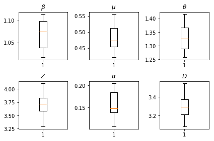
हमारे अनुमानों के परिणाम। सभी वैश्विक पैरामीटर हमारे भर में अपने भिन्नता दिखाने के लिए हम अधिकतम संभावना मूल्यों साजिश num_batches अनुमान के स्वतंत्र रन। यह पूरक सामग्री में तालिका S1 से मेल खाती है।
fig, axs = plt.subplots(2, 3)
axs[0, 0].boxplot(best_parameters.documented_infectious_tx_rate,
                  whis=(2.5,97.5), sym='')
axs[0, 0].set_title(r'$\beta$')

axs[0, 1].boxplot(best_parameters.undocumented_infectious_tx_relative_rate,
                  whis=(2.5,97.5), sym='')
axs[0, 1].set_title(r'$\mu$')

axs[0, 2].boxplot(best_parameters.intercity_underreporting_factor,
                  whis=(2.5,97.5), sym='')
axs[0, 2].set_title(r'$\theta$')

axs[1, 0].boxplot(best_parameters.average_latency_period,
                  whis=(2.5,97.5), sym='')
axs[1, 0].set_title(r'$Z$')

axs[1, 1].boxplot(best_parameters.fraction_of_documented_infections,
                  whis=(2.5,97.5), sym='')
axs[1, 1].set_title(r'$\alpha$')

axs[1, 2].boxplot(best_parameters.average_infection_duration,
                  whis=(2.5,97.5), sym='')
axs[1, 2].set_title(r'$D$')
plt.tight_layout()