
| | |  GitHub पर स्रोत देखें GitHub पर स्रोत देखें | |
यह ट्यूटोरियल क्वांटम सर्किट के अपेक्षित मूल्यों के लिए ग्रेडिएंट कैलकुलेशन एल्गोरिदम की खोज करता है।
एक क्वांटम सर्किट में एक निश्चित अवलोकन के अपेक्षा मूल्य के ढाल की गणना करना एक शामिल प्रक्रिया है। ऑब्जर्वेबल्स के उम्मीद मूल्यों में विश्लेषणात्मक ग्रेडिएंट फ़ार्मुलों होने की विलासिता नहीं होती है जो हमेशा लिखने में आसान होते हैं - पारंपरिक मशीन लर्निंग ट्रांसफ़ॉर्मेशन जैसे कि मैट्रिक्स गुणन या वेक्टर जोड़ के विपरीत जिसमें विश्लेषणात्मक ग्रेडिएंट फ़ार्मुले होते हैं जिन्हें लिखना आसान होता है। नतीजतन, अलग-अलग परिदृश्यों के लिए अलग-अलग क्वांटम ग्रेडिएंट गणना विधियां काम में आती हैं। यह ट्यूटोरियल दो अलग-अलग विभेदन योजनाओं की तुलना और इसके विपरीत है।
सेट अप
pip install tensorflow==2.7.0
TensorFlow क्वांटम स्थापित करें:
pip install tensorflow-quantum
# Update package resources to account for version changes.
import importlib, pkg_resources
importlib.reload(pkg_resources)
<module 'pkg_resources' from '/tmpfs/src/tf_docs_env/lib/python3.7/site-packages/pkg_resources/__init__.py'>
अब TensorFlow और मॉड्यूल निर्भरताएँ आयात करें:
import tensorflow as tf
import tensorflow_quantum as tfq

import cirq
import sympy
import numpy as np

# visualization tools
%matplotlib inline
import matplotlib.pyplot as plt
from cirq.contrib.svg import SVGCircuit
2022-02-04 12:25:24.733670: E tensorflow/stream_executor/cuda/cuda_driver.cc:271] failed call to cuInit: CUDA_ERROR_NO_DEVICE: no CUDA-capable device is detected
1. प्रारंभिक
आइए क्वांटम सर्किट के लिए ढाल गणना की धारणा को थोड़ा और ठोस बनाएं। मान लीजिए कि आपके पास इस तरह एक पैरामीटरयुक्त सर्किट है:
qubit = cirq.GridQubit(0, 0)
my_circuit = cirq.Circuit(cirq.Y(qubit)**sympy.Symbol('alpha'))
SVGCircuit(my_circuit)
findfont: Font family ['Arial'] not found. Falling back to DejaVu Sans.

एक नमूदार के साथ:
pauli_x = cirq.X(qubit)
pauli_x
cirq.X(cirq.GridQubit(0, 0))
इस ऑपरेटर को देखकर आप जानते हैं कि \(⟨Y(\alpha)| X | Y(\alpha)⟩ = \sin(\pi \alpha)\)
def my_expectation(op, alpha):
    """Compute ⟨Y(alpha)| `op` | Y(alpha)⟩"""
    params = {'alpha': alpha}
    sim = cirq.Simulator()
    final_state_vector = sim.simulate(my_circuit, params).final_state_vector
    return op.expectation_from_state_vector(final_state_vector, {qubit: 0}).real


my_alpha = 0.3
print("Expectation=", my_expectation(pauli_x, my_alpha))
print("Sin Formula=", np.sin(np.pi * my_alpha))
Expectation= 0.80901700258255
Sin Formula= 0.8090169943749475
और यदि आप \(f_{1}(\alpha) = ⟨Y(\alpha)| X | Y(\alpha)⟩\) को परिभाषित करते हैं तो \(f_{1}^{'}(\alpha) = \pi \cos(\pi \alpha)\)। आइए इसे जांचें:
def my_grad(obs, alpha, eps=0.01):
    grad = 0
    f_x = my_expectation(obs, alpha)
    f_x_prime = my_expectation(obs, alpha + eps)
    return ((f_x_prime - f_x) / eps).real


print('Finite difference:', my_grad(pauli_x, my_alpha))
print('Cosine formula:   ', np.pi * np.cos(np.pi * my_alpha))
Finite difference: 1.8063604831695557
Cosine formula:    1.8465818304904567
2. एक विभेदक की आवश्यकता
बड़े सर्किट के साथ, आप हमेशा एक सूत्र के लिए इतने भाग्यशाली नहीं होंगे जो किसी दिए गए क्वांटम सर्किट के ग्रेडियेंट की सटीक गणना करता है। इस घटना में कि एक सरल सूत्र ग्रेडिएंट की गणना के लिए पर्याप्त नहीं है, tfq.differentiators.Differentiator वर्ग आपको अपने सर्किट के ग्रेडिएंट की गणना के लिए एल्गोरिदम को परिभाषित करने की अनुमति देता है। उदाहरण के लिए आप उपरोक्त उदाहरण को TensorFlow क्वांटम (TFQ) में फिर से बना सकते हैं:
expectation_calculation = tfq.layers.Expectation(
    differentiator=tfq.differentiators.ForwardDifference(grid_spacing=0.01))

expectation_calculation(my_circuit,
                        operators=pauli_x,
                        symbol_names=['alpha'],
                        symbol_values=[[my_alpha]])
<tf.Tensor: shape=(1, 1), dtype=float32, numpy=array([[0.80901706]], dtype=float32)>
हालाँकि, यदि आप नमूने के आधार पर अनुमान लगाने की अपेक्षा पर स्विच करते हैं (एक सच्चे उपकरण पर क्या होगा) मान थोड़ा बदल सकते हैं। इसका मतलब है कि अब आपके पास एक अपूर्ण अनुमान है:
sampled_expectation_calculation = tfq.layers.SampledExpectation(
    differentiator=tfq.differentiators.ForwardDifference(grid_spacing=0.01))

sampled_expectation_calculation(my_circuit,
                                operators=pauli_x,
                                repetitions=500,
                                symbol_names=['alpha'],
                                symbol_values=[[my_alpha]])
<tf.Tensor: shape=(1, 1), dtype=float32, numpy=array([[0.836]], dtype=float32)>
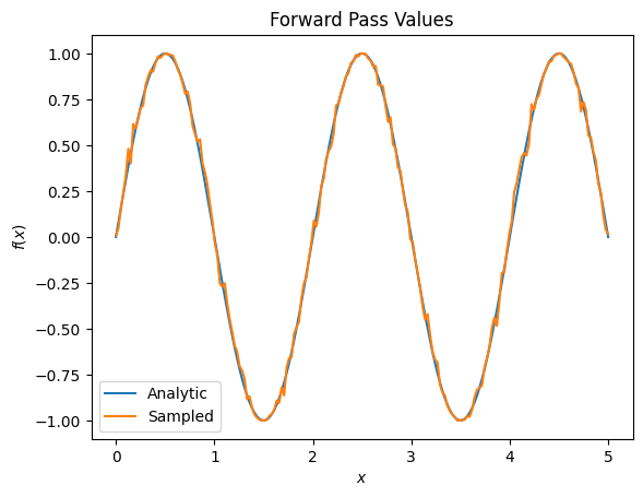
जब ग्रेडिएंट की बात आती है तो यह एक गंभीर सटीकता की समस्या में तेजी से जुड़ सकता है:
# Make input_points = [batch_size, 1] array.
input_points = np.linspace(0, 5, 200)[:, np.newaxis].astype(np.float32)
exact_outputs = expectation_calculation(my_circuit,
                                        operators=pauli_x,
                                        symbol_names=['alpha'],
                                        symbol_values=input_points)
imperfect_outputs = sampled_expectation_calculation(my_circuit,
                                                    operators=pauli_x,
                                                    repetitions=500,
                                                    symbol_names=['alpha'],
                                                    symbol_values=input_points)
plt.title('Forward Pass Values')
plt.xlabel('$x$')
plt.ylabel('$f(x)$')
plt.plot(input_points, exact_outputs, label='Analytic')
plt.plot(input_points, imperfect_outputs, label='Sampled')
plt.legend()
<matplotlib.legend.Legend at 0x7ff07d556190>प्लेसहोल्डर33
# Gradients are a much different story.
values_tensor = tf.convert_to_tensor(input_points)

with tf.GradientTape() as g:
    g.watch(values_tensor)
    exact_outputs = expectation_calculation(my_circuit,
                                            operators=pauli_x,
                                            symbol_names=['alpha'],
                                            symbol_values=values_tensor)
analytic_finite_diff_gradients = g.gradient(exact_outputs, values_tensor)

with tf.GradientTape() as g:
    g.watch(values_tensor)
    imperfect_outputs = sampled_expectation_calculation(
        my_circuit,
        operators=pauli_x,
        repetitions=500,
        symbol_names=['alpha'],
        symbol_values=values_tensor)
sampled_finite_diff_gradients = g.gradient(imperfect_outputs, values_tensor)

plt.title('Gradient Values')
plt.xlabel('$x$')
plt.ylabel('$f^{\'}(x)$')
plt.plot(input_points, analytic_finite_diff_gradients, label='Analytic')
plt.plot(input_points, sampled_finite_diff_gradients, label='Sampled')
plt.legend()
<matplotlib.legend.Legend at 0x7ff07adb8dd0>
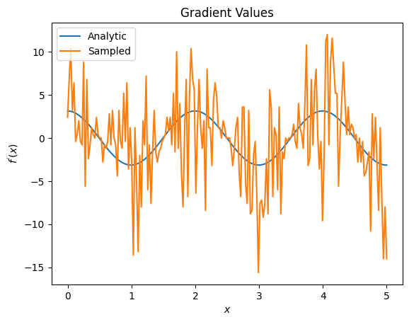
यहां आप देख सकते हैं कि हालांकि परिमित अंतर सूत्र विश्लेषणात्मक मामले में खुद को ढालों की गणना करने के लिए तेज़ है, जब नमूना आधारित विधियों की बात आती है तो यह बहुत शोर था। यह सुनिश्चित करने के लिए अधिक सावधान तकनीकों का उपयोग किया जाना चाहिए कि एक अच्छे ग्रेडिएंट की गणना की जा सके। इसके बाद आप एक बहुत धीमी तकनीक देखेंगे जो विश्लेषणात्मक अपेक्षा ढाल गणना के लिए उपयुक्त नहीं होगी, लेकिन वास्तविक दुनिया के नमूना आधारित मामले में काफी बेहतर प्रदर्शन करती है:
# A smarter differentiation scheme.
gradient_safe_sampled_expectation = tfq.layers.SampledExpectation(
    differentiator=tfq.differentiators.ParameterShift())

with tf.GradientTape() as g:
    g.watch(values_tensor)
    imperfect_outputs = gradient_safe_sampled_expectation(
        my_circuit,
        operators=pauli_x,
        repetitions=500,
        symbol_names=['alpha'],
        symbol_values=values_tensor)

sampled_param_shift_gradients = g.gradient(imperfect_outputs, values_tensor)

plt.title('Gradient Values')
plt.xlabel('$x$')
plt.ylabel('$f^{\'}(x)$')
plt.plot(input_points, analytic_finite_diff_gradients, label='Analytic')
plt.plot(input_points, sampled_param_shift_gradients, label='Sampled')
plt.legend()
<matplotlib.legend.Legend at 0x7ff07ad9ff90>
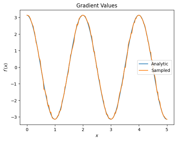
ऊपर से आप देख सकते हैं कि विशेष शोध परिदृश्यों के लिए कुछ विभेदकों का सर्वोत्तम उपयोग किया जाता है। सामान्य तौर पर, धीमी नमूना-आधारित विधियां जो डिवाइस के शोर आदि के लिए मजबूत होती हैं, अधिक "वास्तविक दुनिया" सेटिंग में एल्गोरिदम का परीक्षण या कार्यान्वयन करते समय बहुत भिन्न होती हैं। परिमित अंतर जैसी तेज़ विधियां विश्लेषणात्मक गणनाओं के लिए बहुत अच्छी हैं और आप उच्च थ्रूपुट चाहते हैं, लेकिन अभी तक आपके एल्गोरिदम की डिवाइस व्यवहार्यता से चिंतित नहीं हैं।
3. एकाधिक वेधशाला
आइए एक दूसरे अवलोकन योग्य का परिचय दें और देखें कि कैसे TensorFlow क्वांटम एकल सर्किट के लिए कई वेधशालाओं का समर्थन करता है।
pauli_z = cirq.Z(qubit)
pauli_z
cirq.Z(cirq.GridQubit(0, 0))
यदि यह अवलोकन योग्य पहले की तरह उसी सर्किट के साथ प्रयोग किया जाता है, तो आपके पास \(f_{2}(\alpha) = ⟨Y(\alpha)| Z | Y(\alpha)⟩ = \cos(\pi \alpha)\) और \(f_{2}^{'}(\alpha) = -\pi \sin(\pi \alpha)\)हैं। त्वरित जांच करें:
test_value = 0.

print('Finite difference:', my_grad(pauli_z, test_value))
print('Sin formula:      ', -np.pi * np.sin(np.pi * test_value))
Finite difference: -0.04934072494506836
Sin formula:       -0.0
यह एक मैच है (काफी करीब)।
अब यदि आप \(g(\alpha) = f_{1}(\alpha) + f_{2}(\alpha)\) को परिभाषित करते हैं तो \(g'(\alpha) = f_{1}^{'}(\alpha) + f^{'}_{2}(\alpha)\)। एक सर्किट के साथ उपयोग करने के लिए TensorFlow क्वांटम में एक से अधिक अवलोकन योग्य परिभाषित करना \(g\)में अधिक शर्तों को जोड़ने के बराबर है।
इसका मतलब यह है कि किसी सर्किट में किसी विशेष प्रतीक का ग्रेडिएंट उस सर्किट पर लागू होने वाले प्रतीक के लिए प्रत्येक अवलोकन के संबंध में ग्रेडिएंट के योग के बराबर होता है। यह TensorFlow ग्रेडिएंट लेने और बैकप्रोपेगेशन के साथ संगत है (जहां आप किसी विशेष प्रतीक के लिए ग्रेडिएंट के रूप में सभी अवलोकनों पर ग्रेडिएंट का योग देते हैं)।
sum_of_outputs = tfq.layers.Expectation(
    differentiator=tfq.differentiators.ForwardDifference(grid_spacing=0.01))

sum_of_outputs(my_circuit,
               operators=[pauli_x, pauli_z],
               symbol_names=['alpha'],
               symbol_values=[[test_value]])
<tf.Tensor: shape=(1, 2), dtype=float32, numpy=array([[1.9106855e-15, 1.0000000e+00]], dtype=float32)>
यहां आप देखते हैं कि पहली प्रविष्टि पाउली एक्स की अपेक्षा है, और दूसरी पाउली जेड की अपेक्षा है। अब जब आप ग्रेडिएंट लेते हैं:
test_value_tensor = tf.convert_to_tensor([[test_value]])

with tf.GradientTape() as g:
    g.watch(test_value_tensor)
    outputs = sum_of_outputs(my_circuit,
                             operators=[pauli_x, pauli_z],
                             symbol_names=['alpha'],
                             symbol_values=test_value_tensor)

sum_of_gradients = g.gradient(outputs, test_value_tensor)

print(my_grad(pauli_x, test_value) + my_grad(pauli_z, test_value))
print(sum_of_gradients.numpy())
3.0917350202798843
[[3.0917213]]
यहां आपने सत्यापित किया है कि प्रत्येक अवलोकन योग्य के लिए ग्रेडिएंट का योग वास्तव में \(\alpha\)का ग्रेडिएंट है। यह व्यवहार सभी TensorFlow क्वांटम विभेदकों द्वारा समर्थित है और बाकी TensorFlow के साथ संगतता में महत्वपूर्ण भूमिका निभाता है।
4. उन्नत उपयोग
सभी विभेदक जो TensorFlow क्वांटम उपवर्ग tfq.differentiators.Differentiator के अंदर मौजूद हैं। एक विभेदक को लागू करने के लिए, एक उपयोगकर्ता को दो इंटरफेस में से एक को लागू करना होगा। मानक get_gradient_circuits को लागू करना है, जो बेस क्लास को बताता है कि ग्रेडिएंट का अनुमान प्राप्त करने के लिए कौन से सर्किट को मापना है। वैकल्पिक रूप से, आप differentiate_analytic और differentiate_sampled को ओवरलोड कर सकते हैं; वर्ग tfq.differentiators.Adjoint इस मार्ग को लेता है।
निम्नलिखित सर्किट के ग्रेडिएंट को लागू करने के लिए TensorFlow क्वांटम का उपयोग करता है। आप पैरामीटर स्थानांतरण के एक छोटे से उदाहरण का उपयोग करेंगे।
ऊपर परिभाषित सर्किट को याद करें, \(|\alpha⟩ = Y^{\alpha}|0⟩\)। पहले की तरह, आप \(X\) अवलोकनीय, \(f(\alpha) = ⟨\alpha|X|\alpha⟩\)के विरुद्ध इस सर्किट के अपेक्षा मान के रूप में एक फ़ंक्शन को परिभाषित कर सकते हैं। इस सर्किट के लिए पैरामीटर शिफ्ट नियमों का उपयोग करके, आप पा सकते हैं कि व्युत्पन्न है
\[\frac{\partial}{\partial \alpha} f(\alpha) = \frac{\pi}{2} f\left(\alpha + \frac{1}{2}\right) - \frac{ \pi}{2} f\left(\alpha - \frac{1}{2}\right)\]
get_gradient_circuits फ़ंक्शन इस व्युत्पन्न के घटकों को लौटाता है।
class MyDifferentiator(tfq.differentiators.Differentiator):
    """A Toy differentiator for <Y^alpha | X |Y^alpha>."""

    def __init__(self):
        pass

    def get_gradient_circuits(self, programs, symbol_names, symbol_values):
        """Return circuits to compute gradients for given forward pass circuits.

        Every gradient on a quantum computer can be computed via measurements
        of transformed quantum circuits.  Here, you implement a custom gradient
        for a specific circuit.  For a real differentiator, you will need to
        implement this function in a more general way.  See the differentiator
        implementations in the TFQ library for examples.
        """

        # The two terms in the derivative are the same circuit...
        batch_programs = tf.stack([programs, programs], axis=1)

        # ... with shifted parameter values.
        shift = tf.constant(1/2)
        forward = symbol_values + shift
        backward = symbol_values - shift
        batch_symbol_values = tf.stack([forward, backward], axis=1)

        # Weights are the coefficients of the terms in the derivative.
        num_program_copies = tf.shape(batch_programs)[0]
        batch_weights = tf.tile(tf.constant([[[np.pi/2, -np.pi/2]]]),
                                [num_program_copies, 1, 1])

        # The index map simply says which weights go with which circuits.
        batch_mapper = tf.tile(
            tf.constant([[[0, 1]]]), [num_program_copies, 1, 1])

        return (batch_programs, symbol_names, batch_symbol_values,
                batch_weights, batch_mapper)
Differentiator बेस क्लास व्युत्पन्न की गणना करने के लिए get_gradient_circuits से लौटाए गए घटकों का उपयोग करता है, जैसा कि आपने ऊपर देखे गए पैरामीटर शिफ्ट फॉर्मूला में किया था। यह नया विभेदक अब मौजूदा tfq.layer ऑब्जेक्ट के साथ उपयोग किया जा सकता है:
custom_dif = MyDifferentiator()
custom_grad_expectation = tfq.layers.Expectation(differentiator=custom_dif)

# Now let's get the gradients with finite diff.
with tf.GradientTape() as g:
    g.watch(values_tensor)
    exact_outputs = expectation_calculation(my_circuit,
                                            operators=[pauli_x],
                                            symbol_names=['alpha'],
                                            symbol_values=values_tensor)

analytic_finite_diff_gradients = g.gradient(exact_outputs, values_tensor)

# Now let's get the gradients with custom diff.
with tf.GradientTape() as g:
    g.watch(values_tensor)
    my_outputs = custom_grad_expectation(my_circuit,
                                         operators=[pauli_x],
                                         symbol_names=['alpha'],
                                         symbol_values=values_tensor)

my_gradients = g.gradient(my_outputs, values_tensor)

plt.subplot(1, 2, 1)
plt.title('Exact Gradient')
plt.plot(input_points, analytic_finite_diff_gradients.numpy())
plt.xlabel('x')
plt.ylabel('f(x)')
plt.subplot(1, 2, 2)
plt.title('My Gradient')
plt.plot(input_points, my_gradients.numpy())
plt.xlabel('x')
Text(0.5, 0, 'x')
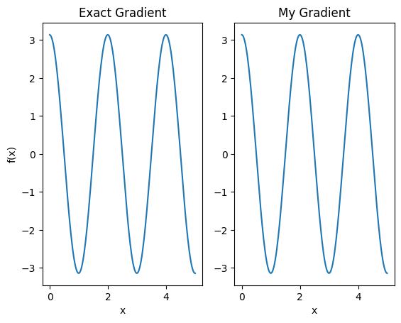
इस नए विभेदक का उपयोग अब अलग-अलग ऑप्स उत्पन्न करने के लिए किया जा सकता है।
# Create a noisy sample based expectation op.
expectation_sampled = tfq.get_sampled_expectation_op(
    cirq.DensityMatrixSimulator(noise=cirq.depolarize(0.01)))

# Make it differentiable with your differentiator:
# Remember to refresh the differentiator before attaching the new op
custom_dif.refresh()
differentiable_op = custom_dif.generate_differentiable_op(
    sampled_op=expectation_sampled)

# Prep op inputs.
circuit_tensor = tfq.convert_to_tensor([my_circuit])
op_tensor = tfq.convert_to_tensor([[pauli_x]])
single_value = tf.convert_to_tensor([[my_alpha]])
num_samples_tensor = tf.convert_to_tensor([[5000]])

with tf.GradientTape() as g:
    g.watch(single_value)
    forward_output = differentiable_op(circuit_tensor, ['alpha'], single_value,
                                       op_tensor, num_samples_tensor)

my_gradients = g.gradient(forward_output, single_value)

print('---TFQ---')
print('Foward:  ', forward_output.numpy())
print('Gradient:', my_gradients.numpy())
print('---Original---')
print('Forward: ', my_expectation(pauli_x, my_alpha))
print('Gradient:', my_grad(pauli_x, my_alpha))
---TFQ---
Foward:   [[0.8016]]
Gradient: [[1.7932211]]
---Original---
Forward:  0.80901700258255
Gradient: 1.8063604831695557