
| | |  GitHub에서 소스 보기 GitHub에서 소스 보기 | |
이 튜토리얼은 양자 회로의 기대값에 대한 기울기 계산 알고리즘을 탐구합니다.
양자 회로에서 관찰 가능한 특정 기대값의 기울기를 계산하는 것은 관련된 과정입니다. 관찰 가능 항목의 기대값은 행렬 곱셈이나 벡터 덧셈과 같이 기록하기 쉬운 분석적 기울기 공식이 있는 기존의 기계 학습 변환과 달리 항상 쓰기 쉬운 분석적 기울기 공식을 갖는 사치품이 아닙니다. 결과적으로 다양한 시나리오에 유용한 다양한 양자 기울기 계산 방법이 있습니다. 이 자습서에서는 두 가지 차별화 체계를 비교하고 대조합니다.
설정
pip install tensorflow==2.7.0
TensorFlow Quantum 설치:
pip install tensorflow-quantum
# Update package resources to account for version changes.
import importlib, pkg_resources
importlib.reload(pkg_resources)
<module 'pkg_resources' from '/tmpfs/src/tf_docs_env/lib/python3.7/site-packages/pkg_resources/__init__.py'>
이제 TensorFlow 및 모듈 종속성을 가져옵니다.
import tensorflow as tf
import tensorflow_quantum as tfq

import cirq
import sympy
import numpy as np

# visualization tools
%matplotlib inline
import matplotlib.pyplot as plt
from cirq.contrib.svg import SVGCircuit
2022-02-04 12:25:24.733670: E tensorflow/stream_executor/cuda/cuda_driver.cc:271] failed call to cuInit: CUDA_ERROR_NO_DEVICE: no CUDA-capable device is detected
1. 예비
양자 회로에 대한 기울기 계산의 개념을 좀 더 구체화합시다. 다음과 같은 매개변수화된 회로가 있다고 가정합니다.
qubit = cirq.GridQubit(0, 0)
my_circuit = cirq.Circuit(cirq.Y(qubit)**sympy.Symbol('alpha'))
SVGCircuit(my_circuit)
findfont: Font family ['Arial'] not found. Falling back to DejaVu Sans.

관찰 가능 항목과 함께:
pauli_x = cirq.X(qubit)
pauli_x
cirq.X(cirq.GridQubit(0, 0))
이 연산자를 보면 \(⟨Y(\alpha)| X | Y(\alpha)⟩ = \sin(\pi \alpha)\)
def my_expectation(op, alpha):
    """Compute ⟨Y(alpha)| `op` | Y(alpha)⟩"""
    params = {'alpha': alpha}
    sim = cirq.Simulator()
    final_state_vector = sim.simulate(my_circuit, params).final_state_vector
    return op.expectation_from_state_vector(final_state_vector, {qubit: 0}).real


my_alpha = 0.3
print("Expectation=", my_expectation(pauli_x, my_alpha))
print("Sin Formula=", np.sin(np.pi * my_alpha))
Expectation= 0.80901700258255
Sin Formula= 0.8090169943749475
\(f_{1}(\alpha) = ⟨Y(\alpha)| X | Y(\alpha)⟩\) 를 정의하면 \(f_{1}^{'}(\alpha) = \pi \cos(\pi \alpha)\)입니다. 이것을 확인해보자:
def my_grad(obs, alpha, eps=0.01):
    grad = 0
    f_x = my_expectation(obs, alpha)
    f_x_prime = my_expectation(obs, alpha + eps)
    return ((f_x_prime - f_x) / eps).real


print('Finite difference:', my_grad(pauli_x, my_alpha))
print('Cosine formula:   ', np.pi * np.cos(np.pi * my_alpha))
Finite difference: 1.8063604831695557
Cosine formula:    1.8465818304904567
2. 차별화 요소의 필요성
더 큰 회로를 사용하면 주어진 양자 회로의 기울기를 정확하게 계산하는 공식을 갖는 것이 항상 운이 좋은 것은 아닙니다. 간단한 공식으로 기울기를 계산하기에 충분하지 않은 경우 tfq.differentiators.Differentiator 클래스를 사용하여 회로의 기울기를 계산하기 위한 알고리즘을 정의할 수 있습니다. 예를 들어 다음을 사용하여 TensorFlow Quantum(TFQ)에서 위의 예를 다시 만들 수 있습니다.
expectation_calculation = tfq.layers.Expectation(
    differentiator=tfq.differentiators.ForwardDifference(grid_spacing=0.01))

expectation_calculation(my_circuit,
                        operators=pauli_x,
                        symbol_names=['alpha'],
                        symbol_values=[[my_alpha]])
<tf.Tensor: shape=(1, 1), dtype=float32, numpy=array([[0.80901706]], dtype=float32)>
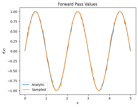
그러나 샘플링을 기반으로 한 기대 추정으로 전환하면(실제 장치에서 발생하는 일) 값이 약간 변경될 수 있습니다. 이것은 이제 불완전한 추정치를 가지고 있음을 의미합니다.
sampled_expectation_calculation = tfq.layers.SampledExpectation(
    differentiator=tfq.differentiators.ForwardDifference(grid_spacing=0.01))

sampled_expectation_calculation(my_circuit,
                                operators=pauli_x,
                                repetitions=500,
                                symbol_names=['alpha'],
                                symbol_values=[[my_alpha]])
<tf.Tensor: shape=(1, 1), dtype=float32, numpy=array([[0.836]], dtype=float32)>
이것은 그라디언트와 관련하여 심각한 정확도 문제로 빠르게 악화될 수 있습니다.
# Make input_points = [batch_size, 1] array.
input_points = np.linspace(0, 5, 200)[:, np.newaxis].astype(np.float32)
exact_outputs = expectation_calculation(my_circuit,
                                        operators=pauli_x,
                                        symbol_names=['alpha'],
                                        symbol_values=input_points)
imperfect_outputs = sampled_expectation_calculation(my_circuit,
                                                    operators=pauli_x,
                                                    repetitions=500,
                                                    symbol_names=['alpha'],
                                                    symbol_values=input_points)
plt.title('Forward Pass Values')
plt.xlabel('$x$')
plt.ylabel('$f(x)$')
plt.plot(input_points, exact_outputs, label='Analytic')
plt.plot(input_points, imperfect_outputs, label='Sampled')
plt.legend()
<matplotlib.legend.Legend at 0x7ff07d556190>
# Gradients are a much different story.
values_tensor = tf.convert_to_tensor(input_points)

with tf.GradientTape() as g:
    g.watch(values_tensor)
    exact_outputs = expectation_calculation(my_circuit,
                                            operators=pauli_x,
                                            symbol_names=['alpha'],
                                            symbol_values=values_tensor)
analytic_finite_diff_gradients = g.gradient(exact_outputs, values_tensor)

with tf.GradientTape() as g:
    g.watch(values_tensor)
    imperfect_outputs = sampled_expectation_calculation(
        my_circuit,
        operators=pauli_x,
        repetitions=500,
        symbol_names=['alpha'],
        symbol_values=values_tensor)
sampled_finite_diff_gradients = g.gradient(imperfect_outputs, values_tensor)

plt.title('Gradient Values')
plt.xlabel('$x$')
plt.ylabel('$f^{\'}(x)$')
plt.plot(input_points, analytic_finite_diff_gradients, label='Analytic')
plt.plot(input_points, sampled_finite_diff_gradients, label='Sampled')
plt.legend()
<matplotlib.legend.Legend at 0x7ff07adb8dd0>
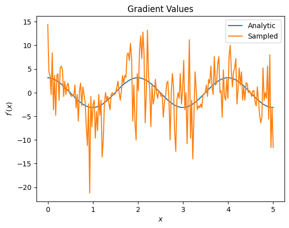
여기에서 유한 차분 공식이 분석 사례에서 기울기 자체를 계산하는 데 빠르지 만 샘플링 기반 방법의 경우 너무 시끄럽다는 것을 알 수 있습니다. 좋은 그래디언트를 계산할 수 있도록 하려면 보다 신중한 기술을 사용해야 합니다. 다음으로 분석적 기대 기울기 계산에는 적합하지 않지만 실제 샘플 기반 사례에서는 훨씬 더 잘 수행되는 훨씬 느린 기술을 살펴보겠습니다.
# A smarter differentiation scheme.
gradient_safe_sampled_expectation = tfq.layers.SampledExpectation(
    differentiator=tfq.differentiators.ParameterShift())

with tf.GradientTape() as g:
    g.watch(values_tensor)
    imperfect_outputs = gradient_safe_sampled_expectation(
        my_circuit,
        operators=pauli_x,
        repetitions=500,
        symbol_names=['alpha'],
        symbol_values=values_tensor)

sampled_param_shift_gradients = g.gradient(imperfect_outputs, values_tensor)

plt.title('Gradient Values')
plt.xlabel('$x$')
plt.ylabel('$f^{\'}(x)$')
plt.plot(input_points, analytic_finite_diff_gradients, label='Analytic')
plt.plot(input_points, sampled_param_shift_gradients, label='Sampled')
plt.legend()
<matplotlib.legend.Legend at 0x7ff07ad9ff90>
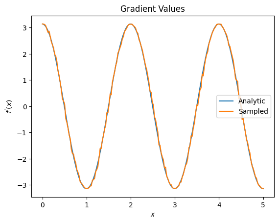
위에서 특정 차별화 요소가 특정 연구 시나리오에 가장 잘 사용됨을 알 수 있습니다. 일반적으로 장치 잡음 등에 강하고 느린 샘플 기반 방법은 "실제" 설정에서 알고리즘을 테스트하거나 구현할 때 큰 차별화 요소입니다. 유한 차분과 같은 더 빠른 방법은 분석 계산에 적합하며 더 높은 처리량을 원하지만 아직 알고리즘의 장치 실행 가능성에 대해서는 관심이 없습니다.
3. 다중 관찰 가능
두 번째 옵저버블을 소개하고 TensorFlow Quantum이 단일 회로에 대해 여러 옵저버블을 지원하는 방법을 살펴보겠습니다.
pauli_z = cirq.Z(qubit)
pauli_z
cirq.Z(cirq.GridQubit(0, 0))
이 관찰 가능 항목이 이전과 동일한 회로와 함께 사용되면 \(f_{2}(\alpha) = ⟨Y(\alpha)| Z | Y(\alpha)⟩ = \cos(\pi \alpha)\) 및 \(f_{2}^{'}(\alpha) = -\pi \sin(\pi \alpha)\)가 있습니다. 빠른 확인 수행:
test_value = 0.

print('Finite difference:', my_grad(pauli_z, test_value))
print('Sin formula:      ', -np.pi * np.sin(np.pi * test_value))
Finite difference: -0.04934072494506836
Sin formula:       -0.0
그것은 경기입니다(충분히 가깝습니다).
이제 \(g(\alpha) = f_{1}(\alpha) + f_{2}(\alpha)\) 을 정의하면 \(g'(\alpha) = f_{1}^{'}(\alpha) + f^{'}_{2}(\alpha)\)입니다. 회로와 함께 사용하기 위해 TensorFlow Quantum에서 둘 이상의 관찰 가능 항목을 정의하는 것은 \(g\)에 더 많은 항을 추가하는 것과 같습니다.
이것은 회로에 있는 특정 기호의 기울기가 해당 회로에 적용된 해당 기호에 대해 관찰 가능한 각각에 대한 기울기의 합과 같다는 것을 의미합니다. 이것은 TensorFlow 그래디언트 가져오기 및 역전파(모든 관찰 가능 항목에 대한 그래디언트의 합계를 특정 기호의 그래디언트로 제공)와 호환됩니다.
sum_of_outputs = tfq.layers.Expectation(
    differentiator=tfq.differentiators.ForwardDifference(grid_spacing=0.01))

sum_of_outputs(my_circuit,
               operators=[pauli_x, pauli_z],
               symbol_names=['alpha'],
               symbol_values=[[test_value]])
<tf.Tensor: shape=(1, 2), dtype=float32, numpy=array([[1.9106855e-15, 1.0000000e+00]], dtype=float32)>
여기에서 첫 번째 항목은 Pauli X의 기대값이고 두 번째 항목은 Pauli Z의 기대값입니다. 이제 그래디언트를 사용할 때:
test_value_tensor = tf.convert_to_tensor([[test_value]])

with tf.GradientTape() as g:
    g.watch(test_value_tensor)
    outputs = sum_of_outputs(my_circuit,
                             operators=[pauli_x, pauli_z],
                             symbol_names=['alpha'],
                             symbol_values=test_value_tensor)

sum_of_gradients = g.gradient(outputs, test_value_tensor)

print(my_grad(pauli_x, test_value) + my_grad(pauli_z, test_value))
print(sum_of_gradients.numpy())
3.0917350202798843
[[3.0917213]]
여기에서 각 옵저버블에 대한 그라디언트의 합이 실제로 \(\alpha\)의 그라디언트임을 확인했습니다. 이 동작은 모든 TensorFlow Quantum 차별화 요소에서 지원되며 나머지 TensorFlow와의 호환성에서 중요한 역할을 합니다.
4. 고급 사용법
TensorFlow Quantum 하위 클래스 tfq.differentiators.Differentiator 내부에 존재하는 모든 차별화 요소입니다. 차별화 요소를 구현하려면 사용자가 두 인터페이스 중 하나를 구현해야 합니다. 표준은 get_gradient_circuits 를 구현하는 것인데, 이는 기울기 추정치를 얻기 위해 측정할 회로를 기본 클래스에 알려줍니다. 또는 differentiate_sampled differentiate_analytic 샘플을 오버로드할 수 있습니다. tfq.differentiators.Adjoint 클래스가 이 경로를 사용합니다.
다음은 TensorFlow Quantum을 사용하여 회로의 기울기를 구현합니다. 매개변수 이동의 작은 예를 사용합니다.
위에서 정의한 회로 \(|\alpha⟩ = Y^{\alpha}|0⟩\)을 기억하십시오. 이전과 마찬가지로 \(X\) 관찰 가능, \(f(\alpha) = ⟨\alpha|X|\alpha⟩\)에 대한 이 회로의 기대값으로 함수를 정의할 수 있습니다. 매개변수 이동 규칙 을 사용하여 이 회로에 대해 도함수가 다음과 같다는 것을 알 수 있습니다.
\[\frac{\partial}{\partial \alpha} f(\alpha) = \frac{\pi}{2} f\left(\alpha + \frac{1}{2}\right) - \frac{ \pi}{2} f\left(\alpha - \frac{1}{2}\right)\]
get_gradient_circuits 함수는 이 도함수의 구성 요소를 반환합니다.
class MyDifferentiator(tfq.differentiators.Differentiator):
    """A Toy differentiator for <Y^alpha | X |Y^alpha>."""

    def __init__(self):
        pass

    def get_gradient_circuits(self, programs, symbol_names, symbol_values):
        """Return circuits to compute gradients for given forward pass circuits.

        Every gradient on a quantum computer can be computed via measurements
        of transformed quantum circuits.  Here, you implement a custom gradient
        for a specific circuit.  For a real differentiator, you will need to
        implement this function in a more general way.  See the differentiator
        implementations in the TFQ library for examples.
        """

        # The two terms in the derivative are the same circuit...
        batch_programs = tf.stack([programs, programs], axis=1)

        # ... with shifted parameter values.
        shift = tf.constant(1/2)
        forward = symbol_values + shift
        backward = symbol_values - shift
        batch_symbol_values = tf.stack([forward, backward], axis=1)

        # Weights are the coefficients of the terms in the derivative.
        num_program_copies = tf.shape(batch_programs)[0]
        batch_weights = tf.tile(tf.constant([[[np.pi/2, -np.pi/2]]]),
                                [num_program_copies, 1, 1])

        # The index map simply says which weights go with which circuits.
        batch_mapper = tf.tile(
            tf.constant([[[0, 1]]]), [num_program_copies, 1, 1])

        return (batch_programs, symbol_names, batch_symbol_values,
                batch_weights, batch_mapper)
Differentiator 기본 클래스는 위에서 본 매개변수 이동 공식에서와 같이 get_gradient_circuits 에서 반환된 구성요소를 사용하여 도함수를 계산합니다. 이 새로운 차별화 요소는 이제 기존 tfq.layer 객체와 함께 사용할 수 있습니다.
custom_dif = MyDifferentiator()
custom_grad_expectation = tfq.layers.Expectation(differentiator=custom_dif)
# Now let's get the gradients with finite diff.
with tf.GradientTape() as g:
g.watch(values_tensor)
exact_outputs = expectation_calculation(my_circuit,
operators=[pauli_x],
symbol_names=['alpha'],
symbol_values=values_tensor)
analytic_finite_diff_gradients = g.gradient(exact_outputs, values_tensor)
# Now let's get the gradients with custom diff.
with tf.GradientTape() as g:
g.watch(values_tensor)
my_outputs = custom_grad_expectation(my_circuit,
operators=[pauli_x],
symbol_names=['alpha'],
symbol_values=values_tensor)
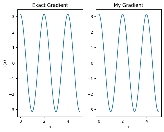
my_gradients = g.gradient(my_outputs, values_tensor)
plt.subplot(1, 2, 1)
plt.title('Exact Gradient')
plt.plot(input_points, analytic_finite_diff_gradients.numpy())
plt.xlabel('x')
plt.ylabel('f(x)')
plt.subplot(1, 2, 2)
plt.title('My Gradient')
plt.plot(input_points, my_gradients.numpy())
plt.xlabel('x')
Text(0.5, 0, 'x')
이제 이 새로운 차별화 요소를 사용하여 차별화 가능한 연산을 생성할 수 있습니다.
# Create a noisy sample based expectation op.
expectation_sampled = tfq.get_sampled_expectation_op(
    cirq.DensityMatrixSimulator(noise=cirq.depolarize(0.01)))

# Make it differentiable with your differentiator:
# Remember to refresh the differentiator before attaching the new op
custom_dif.refresh()
differentiable_op = custom_dif.generate_differentiable_op(
    sampled_op=expectation_sampled)

# Prep op inputs.
circuit_tensor = tfq.convert_to_tensor([my_circuit])
op_tensor = tfq.convert_to_tensor([[pauli_x]])
single_value = tf.convert_to_tensor([[my_alpha]])
num_samples_tensor = tf.convert_to_tensor([[5000]])

with tf.GradientTape() as g:
    g.watch(single_value)
    forward_output = differentiable_op(circuit_tensor, ['alpha'], single_value,
                                       op_tensor, num_samples_tensor)

my_gradients = g.gradient(forward_output, single_value)

print('---TFQ---')
print('Foward:  ', forward_output.numpy())
print('Gradient:', my_gradients.numpy())
print('---Original---')
print('Forward: ', my_expectation(pauli_x, my_alpha))
print('Gradient:', my_grad(pauli_x, my_alpha))
---TFQ---
Foward:   [[0.8016]]
Gradient: [[1.7932211]]
---Original---
Forward:  0.80901700258255
Gradient: 1.8063604831695557