
| | |  GitHub에서 소스 보기 GitHub에서 소스 보기 | |
이 튜토리얼은 기존 신경망이 큐비트 보정 오류를 수정하는 방법을 학습하는 방법을 보여줍니다. NISQ(Noisy Intermediate Scale Quantum) 회로를 생성, 편집 및 호출하는 Python 프레임워크인 Cirq 를 소개하고 Cirq가 TensorFlow Quantum과 인터페이스하는 방법을 보여줍니다.
설정
pip install tensorflow==2.7.0
TensorFlow Quantum 설치:
pip install tensorflow-quantum
# Update package resources to account for version changes.
import importlib, pkg_resources
importlib.reload(pkg_resources)
<module 'pkg_resources' from '/tmpfs/src/tf_docs_env/lib/python3.7/site-packages/pkg_resources/__init__.py'>
이제 TensorFlow 및 모듈 종속성을 가져옵니다.
import tensorflow as tf
import tensorflow_quantum as tfq

import cirq
import sympy
import numpy as np

# visualization tools
%matplotlib inline
import matplotlib.pyplot as plt
from cirq.contrib.svg import SVGCircuit
2022-02-04 12:27:31.677071: E tensorflow/stream_executor/cuda/cuda_driver.cc:271] failed call to cuInit: CUDA_ERROR_NO_DEVICE: no CUDA-capable device is detected
1. 기본
1.1 Cirq 및 매개변수화된 양자 회로
TensorFlow Quantum(TFQ)을 살펴보기 전에 Cirq 의 몇 가지 기본 사항을 살펴보겠습니다. Cirq는 Google의 양자 컴퓨팅을 위한 Python 라이브러리입니다. 이를 사용하여 정적 및 매개변수화된 게이트를 포함한 회로를 정의합니다.
Cirq는 SymPy 기호를 사용하여 자유 매개변수를 나타냅니다.
a, b = sympy.symbols('a b')
다음 코드는 매개변수를 사용하여 2큐비트 회로를 생성합니다.
# Create two qubits
q0, q1 = cirq.GridQubit.rect(1, 2)

# Create a circuit on these qubits using the parameters you created above.
circuit = cirq.Circuit(
    cirq.rx(a).on(q0),
    cirq.ry(b).on(q1), cirq.CNOT(control=q0, target=q1))

SVGCircuit(circuit)
findfont: Font family ['Arial'] not found. Falling back to DejaVu Sans.

회로를 평가하려면 cirq.Simulator 인터페이스를 사용할 수 있습니다. cirq.ParamResolver 개체를 전달하여 회로의 자유 매개변수를 특정 숫자로 바꿉니다. 다음 코드는 매개변수화된 회로의 원시 상태 벡터 출력을 계산합니다.
# Calculate a state vector with a=0.5 and b=-0.5.
resolver = cirq.ParamResolver({a: 0.5, b: -0.5})
output_state_vector = cirq.Simulator().simulate(circuit, resolver).final_state_vector
output_state_vector
array([ 0.9387913 +0.j        , -0.23971277+0.j        ,

        0.        +0.06120872j,  0.        -0.23971277j], dtype=complex64)
상태 벡터는 시뮬레이션 외부에서 직접 액세스할 수 없습니다(위의 출력에서 복소수 참고). 물리적으로 현실적이려면 상태 벡터를 기존 컴퓨터가 이해할 수 있는 실수로 변환하는 측정값을 지정해야 합니다. Cirq는 Pauli 연산자 \(\hat{X}\), \(\hat{Y}\)및 \(\hat{Z}\)의 조합을 사용하여 측정값을 지정합니다. 예를 들어 다음 코드는 방금 시뮬레이션한 상태 벡터에서 l10n \(\hat{Z}_0\) 및 \(\frac{1}{2}\hat{Z}_0 + \hat{X}_1\) 를 측정합니다.
z0 = cirq.Z(q0)

qubit_map={q0: 0, q1: 1}

z0.expectation_from_state_vector(output_state_vector, qubit_map).real
0.8775825500488281
z0x1 = 0.5 * z0 + cirq.X(q1)

z0x1.expectation_from_state_vector(output_state_vector, qubit_map).real
-0.04063427448272705
1.2 텐서로서의 양자 회로
TensorFlow Quantum(TFQ)은 Cirq 객체를 텐서로 변환하는 함수인 tfq.convert_to_tensor 를 제공합니다. 이를 통해 Cirq 개체를 양자 레이어 및 양자 작업 으로 보낼 수 있습니다. 함수는 Cirq Circuits 및 Cirq Paulis의 목록 또는 배열에서 호출할 수 있습니다.
# Rank 1 tensor containing 1 circuit.
circuit_tensor = tfq.convert_to_tensor([circuit])

print(circuit_tensor.shape)
print(circuit_tensor.dtype)
(1,)
<dtype: 'string'>
이것은 Cirq 객체를 tfq 연산이 필요에 따라 디코딩하는 tf.string 텐서로 인코딩합니다.
# Rank 1 tensor containing 2 Pauli operators.
pauli_tensor = tfq.convert_to_tensor([z0, z0x1])
pauli_tensor.shape
TensorShape([2])
1.3 일괄 회로 시뮬레이션
TFQ는 기대값, 샘플 및 상태 벡터를 계산하는 방법을 제공합니다. 지금은 기대값 에 집중해 보겠습니다.
기대값을 계산하기 위한 최상위 인터페이스는 tfq.layers.Expectation 레이어이며 tf.keras.Layer 입니다. 가장 단순한 형태로 이 레이어는 많은 cirq.ParamResolvers 에 대해 매개변수화된 회로를 시뮬레이션하는 것과 같습니다. 그러나 TFQ는 TensorFlow 의미 체계에 따라 일괄 처리를 허용하고 효율적인 C++ 코드를 사용하여 회로를 시뮬레이션합니다.
우리 a 및 b 매개변수를 대체할 값 배치를 작성하십시오.
batch_vals = np.array(np.random.uniform(0, 2 * np.pi, (5, 2)), dtype=np.float32)
Cirq의 매개변수 값에 대한 일괄 회로 실행에는 루프가 필요합니다.
cirq_results = []
cirq_simulator = cirq.Simulator()

for vals in batch_vals:
    resolver = cirq.ParamResolver({a: vals[0], b: vals[1]})
    final_state_vector = cirq_simulator.simulate(circuit, resolver).final_state_vector
    cirq_results.append(
        [z0.expectation_from_state_vector(final_state_vector, {
            q0: 0,
            q1: 1
        }).real])

print('cirq batch results: \n {}'.format(np.array(cirq_results)))
cirq batch results:
 [[-0.66652703]
 [ 0.49764055]
 [ 0.67326665]
 [-0.95549959]
 [-0.81297827]]
TFQ에서는 동일한 작업이 단순화됩니다.
tfq.layers.Expectation()(circuit,
                         symbol_names=[a, b],
                         symbol_values=batch_vals,
                         operators=z0)
<tf.Tensor: shape=(5, 1), dtype=float32, numpy=
array([[-0.666526  ],
       [ 0.49764216],
       [ 0.6732664 ],
       [-0.9554999 ],
       [-0.8129788 ]], dtype=float32)>
2. 하이브리드 양자-고전 최적화
이제 기본 사항을 확인했으므로 TensorFlow Quantum을 사용하여 하이브리드 양자-고전 신경망 을 구성해 보겠습니다. 단일 큐비트를 제어하기 위해 고전적인 신경망을 훈련할 것입니다. 제어는 0 또는 1 상태에서 큐비트를 올바르게 준비하도록 최적화되어 시뮬레이션된 시스템 보정 오류를 극복합니다. 이 그림은 아키텍처를 보여줍니다.
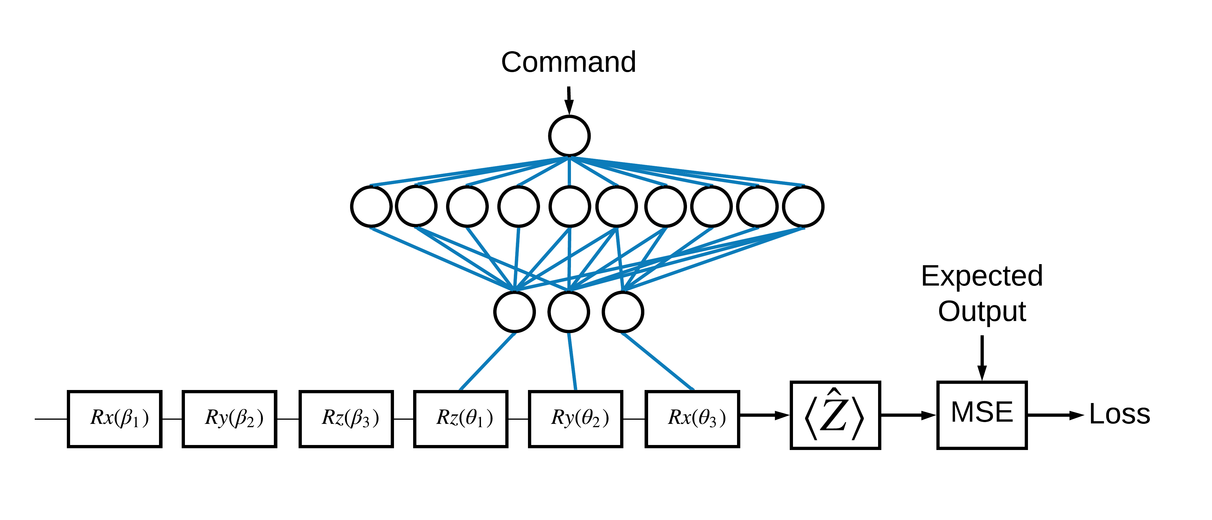
신경망이 없어도 이것은 해결하기 쉬운 문제이지만 주제는 TFQ를 사용하여 해결할 수 있는 실제 양자 제어 문제와 유사합니다. tf.keras.Model 내부의 tfq.layers.ControlledPQC (매개변수 양자 회로) 계층을 사용하는 양자 고전 계산의 종단 간 예제를 보여줍니다.
이 튜토리얼의 구현을 위해 이 아키텍처는 세 부분으로 나뉩니다.
- 입력 회로 또는 데이터 포인트 회로 : 처음 세 개의 \(R\) 게이트.
- 제어된 회로 : 다른 3개의 \(R\) 게이트.
- 컨트롤러 : 제어되는 회로의 매개변수를 설정하는 고전적인 신경망.
2.1 제어 회로 정의
위 그림과 같이 학습 가능한 단일 비트 회전을 정의합니다. 이것은 우리가 제어하는 회로에 해당합니다.
# Parameters that the classical NN will feed values into.
control_params = sympy.symbols('theta_1 theta_2 theta_3')

# Create the parameterized circuit.
qubit = cirq.GridQubit(0, 0)
model_circuit = cirq.Circuit(
    cirq.rz(control_params[0])(qubit),
    cirq.ry(control_params[1])(qubit),
    cirq.rx(control_params[2])(qubit))

SVGCircuit(model_circuit)

2.2 컨트롤러
이제 컨트롤러 네트워크를 정의합니다.
# The classical neural network layers.
controller = tf.keras.Sequential([
    tf.keras.layers.Dense(10, activation='elu'),
    tf.keras.layers.Dense(3)
])
명령 배치가 주어지면 컨트롤러는 제어되는 회로에 대한 제어 신호 배치를 출력합니다.
컨트롤러는 무작위로 초기화되므로 이러한 출력은 아직 유용하지 않습니다.
controller(tf.constant([[0.0],[1.0]])).numpy()
array([[0.        , 0.        , 0.        ],
       [0.5815686 , 0.21376055, 0.57181627]], dtype=float32)
2.3 컨트롤러를 회로에 연결
tfq 를 사용하여 컨트롤러를 제어되는 회로에 단일 keras.Model 로 연결합니다.
이 스타일의 모델 정의에 대한 자세한 내용은 Keras Functional API 가이드 를 참조하세요.
먼저 모델에 대한 입력을 정의합니다.
# This input is the simulated miscalibration that the model will learn to correct.
circuits_input = tf.keras.Input(shape=(),
                                # The circuit-tensor has dtype `tf.string`
                                dtype=tf.string,
                                name='circuits_input')

# Commands will be either `0` or `1`, specifying the state to set the qubit to.
commands_input = tf.keras.Input(shape=(1,),
                                dtype=tf.dtypes.float32,
                                name='commands_input')
그런 다음 해당 입력에 작업을 적용하여 계산을 정의합니다.
dense_2 = controller(commands_input)

# TFQ layer for classically controlled circuits.
expectation_layer = tfq.layers.ControlledPQC(model_circuit,
                                             # Observe Z
                                             operators = cirq.Z(qubit))
expectation = expectation_layer([circuits_input, dense_2])
이제 이 계산을 tf.keras.Model 로 패키징합니다.
# The full Keras model is built from our layers.
model = tf.keras.Model(inputs=[circuits_input, commands_input],
                       outputs=expectation)
네트워크 아키텍처는 아래 모델의 플롯으로 표시됩니다. 이 모델 플롯을 아키텍처 다이어그램과 비교하여 정확성을 확인합니다.
tf.keras.utils.plot_model(model, show_shapes=True, dpi=70)
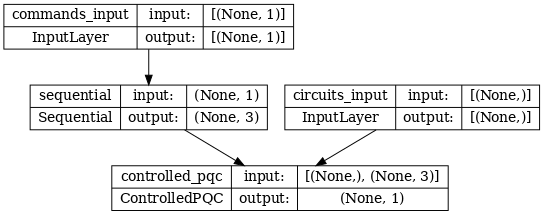
이 모델은 컨트롤러에 대한 명령과 컨트롤러가 수정하려고 시도하는 출력의 입력 회로라는 두 가지 입력을 받습니다.
2.4 데이터세트
모델은 각 명령에 대해 \(\hat{Z}\) 의 정확한 측정 값을 출력하려고 시도합니다. 명령과 올바른 값은 아래에 정의되어 있습니다.
# The command input values to the classical NN.
commands = np.array([[0], [1]], dtype=np.float32)

# The desired Z expectation value at output of quantum circuit.
expected_outputs = np.array([[1], [-1]], dtype=np.float32)
이것은 이 작업에 대한 전체 교육 데이터 세트가 아닙니다. 데이터 세트의 각 데이터 포인트에는 입력 회로도 필요합니다.
2.4 입력 회로 정의
아래의 입력 회로는 모델이 수정하도록 학습할 임의의 오교정을 정의합니다.
random_rotations = np.random.uniform(0, 2 * np.pi, 3)
noisy_preparation = cirq.Circuit(
  cirq.rx(random_rotations[0])(qubit),
  cirq.ry(random_rotations[1])(qubit),
  cirq.rz(random_rotations[2])(qubit)
)
datapoint_circuits = tfq.convert_to_tensor([
  noisy_preparation
] * 2)  # Make two copied of this circuit
각 데이터 포인트에 대해 하나씩 2개의 회로 복사본이 있습니다.
datapoint_circuits.shape
TensorShape([2])
2.5 훈련
정의된 입력으로 tfq 모델을 테스트할 수 있습니다.
model([datapoint_circuits, commands]).numpy()
array([[0.95853525],
       [0.6272128 ]], dtype=float32)
이제 표준 교육 프로세스를 실행하여 이러한 값을 expected_outputs 출력으로 조정합니다.
optimizer = tf.keras.optimizers.Adam(learning_rate=0.05)
loss = tf.keras.losses.MeanSquaredError()
model.compile(optimizer=optimizer, loss=loss)
history = model.fit(x=[datapoint_circuits, commands],
                    y=expected_outputs,
                    epochs=30,
                    verbose=0)
plt.plot(history.history['loss'])
plt.title("Learning to Control a Qubit")
plt.xlabel("Iterations")
plt.ylabel("Error in Control")
plt.show()
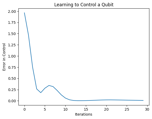
이 플롯에서 신경망이 체계적인 오보정을 극복하는 방법을 배웠음을 알 수 있습니다.
2.6 출력 확인
이제 훈련된 모델을 사용하여 큐비트 보정 오류를 수정합니다. Cirq와 함께:
def check_error(command_values, desired_values):
  """Based on the value in `command_value` see how well you could prepare
  the full circuit to have `desired_value` when taking expectation w.r.t. Z."""
  params_to_prepare_output = controller(command_values).numpy()
  full_circuit = noisy_preparation + model_circuit

  # Test how well you can prepare a state to get expectation the expectation
  # value in `desired_values`
  for index in [0, 1]:
    state = cirq_simulator.simulate(
        full_circuit,
        {s:v for (s,v) in zip(control_params, params_to_prepare_output[index])}
    ).final_state_vector
    expt = cirq.Z(qubit).expectation_from_state_vector(state, {qubit: 0}).real
    print(f'For a desired output (expectation) of {desired_values[index]} with'
          f' noisy preparation, the controller\nnetwork found the following '
          f'values for theta: {params_to_prepare_output[index]}\nWhich gives an'
          f' actual expectation of: {expt}\n')


check_error(commands, expected_outputs)
For a desired output (expectation) of [1.] with noisy preparation, the controller
network found the following values for theta: [-0.6788422   0.3395225  -0.59394693]
Which gives an actual expectation of: 0.9171845316886902

For a desired output (expectation) of [-1.] with noisy preparation, the controller
network found the following values for theta: [-5.203663   -0.29528576  3.2887425 ]
Which gives an actual expectation of: -0.9511058330535889
훈련 중 손실 함수의 값은 모델이 얼마나 잘 학습하고 있는지에 대한 대략적인 아이디어를 제공합니다. 손실이 낮을수록 위 셀의 기대값이 desired_values 에 더 가깝습니다. 매개변수 값에 관심이 없다면 항상 tfq 를 사용하여 위의 출력을 확인할 수 있습니다.
model([datapoint_circuits, commands])
<tf.Tensor: shape=(2, 1), dtype=float32, numpy=
array([[ 0.91718477],
       [-0.9511056 ]], dtype=float32)>
3 다른 연산자의 고유 상태를 준비하는 방법 학습
1과 0에 해당하는 \(\pm \hat{Z}\) 고유 상태의 선택은 임의적이었습니다. 1이 \(+ \hat{Z}\) \(-\hat{X}\) 상태에 해당하도록 쉽게 원할 수 있습니다. 이를 수행하는 한 가지 방법은 아래 그림에 표시된 대로 각 명령에 대해 다른 측정 연산자를 지정하는 것입니다.

이를 위해서는 tfq.layers.Expectation 을 사용해야 합니다. 이제 입력에 회로, 명령 및 연산자의 세 가지 개체가 포함됩니다. 출력은 여전히 기대값입니다.
3.1 새로운 모델 정의
이 작업을 수행하기 위한 모델을 살펴보겠습니다.
# Define inputs.
commands_input = tf.keras.layers.Input(shape=(1),
                                       dtype=tf.dtypes.float32,
                                       name='commands_input')
circuits_input = tf.keras.Input(shape=(),
                                # The circuit-tensor has dtype `tf.string`
                                dtype=tf.dtypes.string,
                                name='circuits_input')
operators_input = tf.keras.Input(shape=(1,),
                                 dtype=tf.dtypes.string,
                                 name='operators_input')
컨트롤러 네트워크는 다음과 같습니다.
# Define classical NN.
controller = tf.keras.Sequential([
    tf.keras.layers.Dense(10, activation='elu'),
    tf.keras.layers.Dense(3)
])
tfq 를 사용하여 회로와 컨트롤러를 단일 keras.Model 로 결합합니다.
dense_2 = controller(commands_input)

# Since you aren't using a PQC or ControlledPQC you must append
# your model circuit onto the datapoint circuit tensor manually.
full_circuit = tfq.layers.AddCircuit()(circuits_input, append=model_circuit)
expectation_output = tfq.layers.Expectation()(full_circuit,
                                              symbol_names=control_params,
                                              symbol_values=dense_2,
                                              operators=operators_input)

# Contruct your Keras model.
two_axis_control_model = tf.keras.Model(
    inputs=[circuits_input, commands_input, operators_input],
    outputs=[expectation_output])
3.2 데이터세트
이제 model_circuit 에 제공하는 각 데이터 포인트에 대해 측정하려는 연산자도 포함합니다.
# The operators to measure, for each command.
operator_data = tfq.convert_to_tensor([[cirq.X(qubit)], [cirq.Z(qubit)]])

# The command input values to the classical NN.
commands = np.array([[0], [1]], dtype=np.float32)

# The desired expectation value at output of quantum circuit.
expected_outputs = np.array([[1], [-1]], dtype=np.float32)
3.3 훈련
이제 새로운 입력과 출력이 있으므로 keras를 사용하여 다시 한 번 훈련할 수 있습니다.
optimizer = tf.keras.optimizers.Adam(learning_rate=0.05)
loss = tf.keras.losses.MeanSquaredError()

two_axis_control_model.compile(optimizer=optimizer, loss=loss)

history = two_axis_control_model.fit(
    x=[datapoint_circuits, commands, operator_data],
    y=expected_outputs,
    epochs=30,
    verbose=1)
Epoch 1/30
1/1 [==============================] - 0s 320ms/step - loss: 2.4404
Epoch 2/30
1/1 [==============================] - 0s 3ms/step - loss: 1.8713
Epoch 3/30
1/1 [==============================] - 0s 3ms/step - loss: 1.1400
Epoch 4/30
1/1 [==============================] - 0s 3ms/step - loss: 0.5071
Epoch 5/30
1/1 [==============================] - 0s 3ms/step - loss: 0.1611
Epoch 6/30
1/1 [==============================] - 0s 3ms/step - loss: 0.0426
Epoch 7/30
1/1 [==============================] - 0s 3ms/step - loss: 0.0117
Epoch 8/30
1/1 [==============================] - 0s 3ms/step - loss: 0.0032
Epoch 9/30
1/1 [==============================] - 0s 2ms/step - loss: 0.0147
Epoch 10/30
1/1 [==============================] - 0s 3ms/step - loss: 0.0452
Epoch 11/30
1/1 [==============================] - 0s 3ms/step - loss: 0.0670
Epoch 12/30
1/1 [==============================] - 0s 3ms/step - loss: 0.0648
Epoch 13/30
1/1 [==============================] - 0s 3ms/step - loss: 0.0471
Epoch 14/30
1/1 [==============================] - 0s 3ms/step - loss: 0.0289
Epoch 15/30
1/1 [==============================] - 0s 3ms/step - loss: 0.0180
Epoch 16/30
1/1 [==============================] - 0s 3ms/step - loss: 0.0138
Epoch 17/30
1/1 [==============================] - 0s 2ms/step - loss: 0.0130
Epoch 18/30
1/1 [==============================] - 0s 3ms/step - loss: 0.0137
Epoch 19/30
1/1 [==============================] - 0s 3ms/step - loss: 0.0148
Epoch 20/30
1/1 [==============================] - 0s 3ms/step - loss: 0.0156
Epoch 21/30
1/1 [==============================] - 0s 3ms/step - loss: 0.0157
Epoch 22/30
1/1 [==============================] - 0s 3ms/step - loss: 0.0149
Epoch 23/30
1/1 [==============================] - 0s 3ms/step - loss: 0.0135
Epoch 24/30
1/1 [==============================] - 0s 3ms/step - loss: 0.0119
Epoch 25/30
1/1 [==============================] - 0s 3ms/step - loss: 0.0100
Epoch 26/30
1/1 [==============================] - 0s 3ms/step - loss: 0.0082
Epoch 27/30
1/1 [==============================] - 0s 3ms/step - loss: 0.0064
Epoch 28/30
1/1 [==============================] - 0s 3ms/step - loss: 0.0047
Epoch 29/30
1/1 [==============================] - 0s 3ms/step - loss: 0.0034
Epoch 30/30
1/1 [==============================] - 0s 3ms/step - loss: 0.0024
plt.plot(history.history['loss'])
plt.title("Learning to Control a Qubit")
plt.xlabel("Iterations")
plt.ylabel("Error in Control")
plt.show()
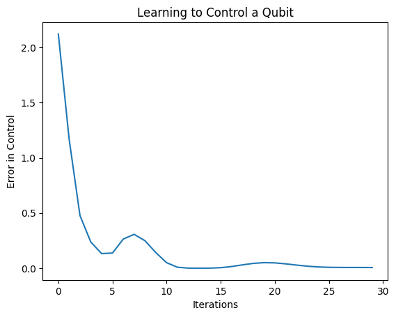
손실 함수가 0으로 떨어졌습니다.
controller 는 독립형 모델로 제공됩니다. 컨트롤러를 호출하고 각 명령 신호에 대한 응답을 확인합니다. 이러한 출력을 random_rotations 의 내용과 올바르게 비교하려면 약간의 작업이 필요합니다.
controller.predict(np.array([0,1]))
array([[3.6335812 , 1.8470774 , 0.71675825],
       [5.3085413 , 0.08116499, 2.8337662 ]], dtype=float32)