
| | |  GitHub에서 소스 보기 GitHub에서 소스 보기 | |
이 튜토리얼은 Farhi et al 에서 사용된 접근 방식과 유사한 MNIST의 단순화된 버전을 분류하기 위해 양자 신경망(QNN)을 구축합니다. 이 고전적인 데이터 문제에 대한 양자 신경망의 성능은 고전적인 신경망과 비교됩니다.
설정
pip install tensorflow==2.7.0
TensorFlow Quantum 설치:
pip install tensorflow-quantum
# Update package resources to account for version changes.
import importlib, pkg_resources
importlib.reload(pkg_resources)
<module 'pkg_resources' from '/tmpfs/src/tf_docs_env/lib/python3.7/site-packages/pkg_resources/__init__.py'>
이제 TensorFlow 및 모듈 종속성을 가져옵니다.
import tensorflow as tf
import tensorflow_quantum as tfq

import cirq
import sympy
import numpy as np
import seaborn as sns
import collections

# visualization tools
%matplotlib inline
import matplotlib.pyplot as plt
from cirq.contrib.svg import SVGCircuit
2022-02-04 12:29:39.759643: E tensorflow/stream_executor/cuda/cuda_driver.cc:271] failed call to cuInit: CUDA_ERROR_NO_DEVICE: no CUDA-capable device is detected
1. 데이터 로드
이 자습서에서는 Farhi et al.에 따라 숫자 3과 6을 구별하는 이진 분류기를 빌드합니다. 이 섹션에서는 다음과 같은 데이터 처리를 다룹니다.
- Keras에서 원시 데이터를 로드합니다.
- 데이터 세트를 3과 6으로만 필터링합니다.
- 양자 컴퓨터에 맞도록 이미지를 축소합니다.
- 모순되는 예를 제거합니다.
- 바이너리 이미지를 Cirq 회로로 변환합니다.
- Cirq 회로를 TensorFlow Quantum 회로로 변환합니다.
1.1 원시 데이터 로드
Keras와 함께 배포된 MNIST 데이터 세트를 로드합니다.
(x_train, y_train), (x_test, y_test) = tf.keras.datasets.mnist.load_data()

# Rescale the images from [0,255] to the [0.0,1.0] range.
x_train, x_test = x_train[..., np.newaxis]/255.0, x_test[..., np.newaxis]/255.0

print("Number of original training examples:", len(x_train))
print("Number of original test examples:", len(x_test))
Downloading data from https://storage.googleapis.com/tensorflow/tf-keras-datasets/mnist.npz
11493376/11490434 [==============================] - 0s 0us/step
11501568/11490434 [==============================] - 0s 0us/step
Number of original training examples: 60000
Number of original test examples: 10000
데이터 세트를 필터링하여 3과 6만 유지하고 다른 클래스는 제거합니다. 동시에 레이블 y 를 부울로 변환합니다. 3 은 True , 6은 False 입니다.
def filter_36(x, y):
    keep = (y == 3) | (y == 6)
    x, y = x[keep], y[keep]
    y = y == 3
    return x,y
x_train, y_train = filter_36(x_train, y_train)
x_test, y_test = filter_36(x_test, y_test)

print("Number of filtered training examples:", len(x_train))
print("Number of filtered test examples:", len(x_test))
Number of filtered training examples: 12049
Number of filtered test examples: 1968
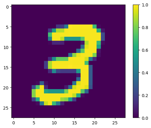
첫 번째 예를 보여줍니다.
print(y_train[0])

plt.imshow(x_train[0, :, :, 0])
plt.colorbar()
True
<matplotlib.colorbar.Colorbar at 0x7fac6ad4bd90>
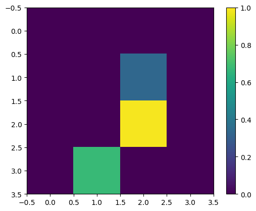
1.2 이미지 축소
28x28의 이미지 크기는 현재 양자 컴퓨터에 비해 너무 큽니다. 이미지 크기를 4x4로 줄입니다.
x_train_small = tf.image.resize(x_train, (4,4)).numpy()
x_test_small = tf.image.resize(x_test, (4,4)).numpy()
다시, 크기 조정 후 첫 번째 훈련 예제를 표시합니다.
print(y_train[0])

plt.imshow(x_train_small[0,:,:,0], vmin=0, vmax=1)
plt.colorbar()
True
<matplotlib.colorbar.Colorbar at 0x7fabf807fe10>
1.3 모순되는 예 제거
섹션 3.3 에서 Farhi et al.의 숫자 구별 학습. , 데이터 세트를 필터링하여 두 클래스에 모두 속하는 것으로 레이블이 지정된 이미지를 제거합니다.
이것은 표준 기계 학습 절차가 아니지만 논문을 따르기 위해 포함됩니다.
def remove_contradicting(xs, ys):
    mapping = collections.defaultdict(set)
    orig_x = {}
    # Determine the set of labels for each unique image:
    for x,y in zip(xs,ys):
       orig_x[tuple(x.flatten())] = x
       mapping[tuple(x.flatten())].add(y)

    new_x = []
    new_y = []
    for flatten_x in mapping:
      x = orig_x[flatten_x]
      labels = mapping[flatten_x]
      if len(labels) == 1:
          new_x.append(x)
          new_y.append(next(iter(labels)))
      else:
          # Throw out images that match more than one label.
          pass

    num_uniq_3 = sum(1 for value in mapping.values() if len(value) == 1 and True in value)
    num_uniq_6 = sum(1 for value in mapping.values() if len(value) == 1 and False in value)
    num_uniq_both = sum(1 for value in mapping.values() if len(value) == 2)

    print("Number of unique images:", len(mapping.values()))
    print("Number of unique 3s: ", num_uniq_3)
    print("Number of unique 6s: ", num_uniq_6)
    print("Number of unique contradicting labels (both 3 and 6): ", num_uniq_both)
    print()
    print("Initial number of images: ", len(xs))
    print("Remaining non-contradicting unique images: ", len(new_x))

    return np.array(new_x), np.array(new_y)
결과 개수는 보고된 값과 거의 일치하지 않지만 정확한 절차는 지정되지 않습니다.
이 시점에서 모순되는 예제 필터링을 적용해도 모델이 모순된 훈련 예제를 수신하는 것을 완전히 막을 수는 없습니다. 다음 단계는 더 많은 충돌을 일으킬 데이터를 이진화합니다.
x_train_nocon, y_train_nocon = remove_contradicting(x_train_small, y_train)
Number of unique images: 10387
Number of unique 3s:  4912
Number of unique 6s:  5426
Number of unique contradicting labels (both 3 and 6):  49

Initial number of images:  12049
Remaining non-contradicting unique images:  10338
1.4 데이터를 양자 회로로 인코딩
양자 컴퓨터를 사용하여 이미지를 처리하기 위해 Farhi et al. 각 픽셀을 큐비트로 표현하는 것이 제안되었으며, 픽셀 값에 따라 상태가 결정됩니다. 첫 번째 단계는 이진 인코딩으로 변환하는 것입니다.
THRESHOLD = 0.5

x_train_bin = np.array(x_train_nocon > THRESHOLD, dtype=np.float32)
x_test_bin = np.array(x_test_small > THRESHOLD, dtype=np.float32)
이 시점에서 모순되는 이미지를 제거하면 193개만 남게 되므로 효과적인 훈련에 충분하지 않을 수 있습니다.
_ = remove_contradicting(x_train_bin, y_train_nocon)
Number of unique images: 193
Number of unique 3s:  80
Number of unique 6s:  69
Number of unique contradicting labels (both 3 and 6):  44

Initial number of images:  10338
Remaining non-contradicting unique images:  149
임계값을 초과하는 값을 가진 픽셀 인덱스의 큐비 \(X\) 게이트를 통해 회전됩니다.
def convert_to_circuit(image):
    """Encode truncated classical image into quantum datapoint."""
    values = np.ndarray.flatten(image)
    qubits = cirq.GridQubit.rect(4, 4)
    circuit = cirq.Circuit()
    for i, value in enumerate(values):
        if value:
            circuit.append(cirq.X(qubits[i]))
    return circuit


x_train_circ = [convert_to_circuit(x) for x in x_train_bin]
x_test_circ = [convert_to_circuit(x) for x in x_test_bin]
다음은 첫 번째 예를 위해 만든 회로입니다(회로 다이어그램에는 게이트가 0인 큐비트가 표시되지 않음).
SVGCircuit(x_train_circ[0])
findfont: Font family ['Arial'] not found. Falling back to DejaVu Sans.

이 회로를 이미지 값이 임계값을 초과하는 인덱스와 비교하십시오.
bin_img = x_train_bin[0,:,:,0]
indices = np.array(np.where(bin_img)).T
indices
array([[2, 2],
       [3, 1]])
다음 Cirq 회로를 tfq 용 텐서로 변환합니다.
x_train_tfcirc = tfq.convert_to_tensor(x_train_circ)
x_test_tfcirc = tfq.convert_to_tensor(x_test_circ)
2. 양자 신경망
이미지를 분류하는 양자 회로 구조에 대한 지침은 거의 없습니다. 분류는 판독 큐비트의 기대치를 기반으로 하기 때문에 Farhi et al. 판독 큐비트가 항상 작동하는 두 개의 큐비트 게이트 사용을 제안합니다. 이것은 픽셀 전체에서 작은 단일 RNN 을 실행하는 것과 어떤 면에서 유사합니다.
2.1 모델 회로 구축
다음 예는 이 계층적 접근 방식을 보여줍니다. 각 계층은 동일한 게이트의 n 인스턴스를 사용하며 각 데이터 큐비트는 판독 큐비트에 작용합니다.
회로에 이러한 게이트 레이어를 추가하는 간단한 클래스로 시작합니다.
class CircuitLayerBuilder():
    def __init__(self, data_qubits, readout):
        self.data_qubits = data_qubits
        self.readout = readout

    def add_layer(self, circuit, gate, prefix):
        for i, qubit in enumerate(self.data_qubits):
            symbol = sympy.Symbol(prefix + '-' + str(i))
            circuit.append(gate(qubit, self.readout)**symbol)
어떻게 보이는지 보려면 예제 회로 레이어를 빌드하십시오.
demo_builder = CircuitLayerBuilder(data_qubits = cirq.GridQubit.rect(4,1),
                                   readout=cirq.GridQubit(-1,-1))

circuit = cirq.Circuit()
demo_builder.add_layer(circuit, gate = cirq.XX, prefix='xx')
SVGCircuit(circuit)

이제 데이터 회로 크기와 일치하는 2계층 모델을 구축하고 준비 및 판독 작업을 포함합니다.
def create_quantum_model():
    """Create a QNN model circuit and readout operation to go along with it."""
    data_qubits = cirq.GridQubit.rect(4, 4)  # a 4x4 grid.
    readout = cirq.GridQubit(-1, -1)         # a single qubit at [-1,-1]
    circuit = cirq.Circuit()

    # Prepare the readout qubit.
    circuit.append(cirq.X(readout))
    circuit.append(cirq.H(readout))

    builder = CircuitLayerBuilder(
        data_qubits = data_qubits,
        readout=readout)

    # Then add layers (experiment by adding more).
    builder.add_layer(circuit, cirq.XX, "xx1")
    builder.add_layer(circuit, cirq.ZZ, "zz1")

    # Finally, prepare the readout qubit.
    circuit.append(cirq.H(readout))

    return circuit, cirq.Z(readout)
model_circuit, model_readout = create_quantum_model()
2.2 모델 회로를 tfq-keras 모델로 래핑
양자 구성 요소로 Keras 모델을 구축합니다. 이 모델은 기존 데이터를 인코딩하는 x_train_circ 에서 "양자 데이터"를 제공받습니다. 매개변수화된 양자 회로 계층인 tfq.layers.PQC 를 사용하여 양자 데이터에서 모델 회로를 훈련합니다.
이러한 이미지를 분류하기 위해 Farhi et al. 매개변수화된 회로에서 판독 큐비트를 예상하는 것을 제안했습니다. 기대값은 1과 -1 사이의 값을 반환합니다.
# Build the Keras model.
model = tf.keras.Sequential([
    # The input is the data-circuit, encoded as a tf.string
    tf.keras.layers.Input(shape=(), dtype=tf.string),
    # The PQC layer returns the expected value of the readout gate, range [-1,1].
    tfq.layers.PQC(model_circuit, model_readout),
])
다음으로, compile 방법을 사용하여 모델에 훈련 절차를 설명합니다.
예상 판독값이 [-1,1] 범위에 있기 때문에 힌지 손실을 최적화하는 것이 다소 자연스럽습니다.
여기서 힌지 손실을 사용하려면 두 가지 작은 조정이 필요합니다. 먼저 경첩 손실에 의해 예상되는 대로 레이블 y_train_nocon 을 부울에서 [-1,1] 로 변환합니다.
y_train_hinge = 2.0*y_train_nocon-1.0
y_test_hinge = 2.0*y_test-1.0
둘째, [-1, 1] 을 hinge_accuracy 레이블 인수 y_true 올바르게 처리하는 사용자 지정 힌지_정확도 측정항목을 사용합니다. tf.losses.BinaryAccuracy(threshold=0.0) 는 y_true 가 부울일 것으로 예상하므로 힌지 손실과 함께 사용할 수 없습니다.
def hinge_accuracy(y_true, y_pred):
    y_true = tf.squeeze(y_true) > 0.0
    y_pred = tf.squeeze(y_pred) > 0.0
    result = tf.cast(y_true == y_pred, tf.float32)

    return tf.reduce_mean(result)
model.compile(
    loss=tf.keras.losses.Hinge(),
    optimizer=tf.keras.optimizers.Adam(),
    metrics=[hinge_accuracy])
print(model.summary())
Model: "sequential"
_________________________________________________________________
 Layer (type)                Output Shape              Param #
=================================================================
 pqc (PQC)                   (None, 1)                 32

=================================================================
Total params: 32
Trainable params: 32
Non-trainable params: 0
_________________________________________________________________
None
양자 모델 훈련
이제 모델을 학습시키십시오. 약 45분이 소요됩니다. 그렇게 오래 기다리지 않으려면 데이터의 작은 하위 집합을 사용하십시오(아래에서 NUM_EXAMPLES=500 설정). 이것은 훈련 중 모델의 진행 상황에 실제로 영향을 미치지 않습니다(단 32개의 매개변수가 있으며 이를 제한하는 데 많은 데이터가 필요하지 않음). 더 적은 수의 예제를 사용하면 훈련이 더 일찍 종료되지만(5분) 유효성 검사 로그에서 진행되고 있음을 보여줄 만큼 충분히 오래 실행됩니다.
EPOCHS = 3
BATCH_SIZE = 32

NUM_EXAMPLES = len(x_train_tfcirc)
x_train_tfcirc_sub = x_train_tfcirc[:NUM_EXAMPLES]
y_train_hinge_sub = y_train_hinge[:NUM_EXAMPLES]
이 모델을 수렴하도록 훈련하면 테스트 세트에서 85% 이상의 정확도를 달성해야 합니다.
qnn_history = model.fit(
      x_train_tfcirc_sub, y_train_hinge_sub,
      batch_size=32,
      epochs=EPOCHS,
      verbose=1,
      validation_data=(x_test_tfcirc, y_test_hinge))

qnn_results = model.evaluate(x_test_tfcirc, y_test)
Epoch 1/3
324/324 [==============================] - 68s 207ms/step - loss: 0.6745 - hinge_accuracy: 0.7719 - val_loss: 0.3959 - val_hinge_accuracy: 0.8004
Epoch 2/3
324/324 [==============================] - 68s 209ms/step - loss: 0.3964 - hinge_accuracy: 0.8291 - val_loss: 0.3498 - val_hinge_accuracy: 0.8997
Epoch 3/3
324/324 [==============================] - 66s 204ms/step - loss: 0.3599 - hinge_accuracy: 0.8854 - val_loss: 0.3395 - val_hinge_accuracy: 0.9042
62/62 [==============================] - 3s 41ms/step - loss: 0.3395 - hinge_accuracy: 0.9042
3. 고전적 신경망
양자 신경망은 이 단순화된 MNIST 문제에 대해 작동하지만 기본 고전 신경망은 이 작업에서 QNN을 쉽게 능가할 수 있습니다. 단일 에포크 후에 기존 신경망은 홀드아웃 세트에서 >98% 정확도를 달성할 수 있습니다.
다음 예에서는 이미지를 서브샘플링하는 대신 전체 28x28 이미지를 사용하여 3-6 분류 문제에 대해 고전적 신경망을 사용합니다. 이것은 테스트 세트의 거의 100% 정확도로 쉽게 수렴됩니다.
def create_classical_model():
    # A simple model based off LeNet from https://keras.io/examples/mnist_cnn/
    model = tf.keras.Sequential()
    model.add(tf.keras.layers.Conv2D(32, [3, 3], activation='relu', input_shape=(28,28,1)))
    model.add(tf.keras.layers.Conv2D(64, [3, 3], activation='relu'))
    model.add(tf.keras.layers.MaxPooling2D(pool_size=(2, 2)))
    model.add(tf.keras.layers.Dropout(0.25))
    model.add(tf.keras.layers.Flatten())
    model.add(tf.keras.layers.Dense(128, activation='relu'))
    model.add(tf.keras.layers.Dropout(0.5))
    model.add(tf.keras.layers.Dense(1))
    return model


model = create_classical_model()
model.compile(loss=tf.keras.losses.BinaryCrossentropy(from_logits=True),
              optimizer=tf.keras.optimizers.Adam(),
              metrics=['accuracy'])

model.summary()
Model: "sequential_1"
_________________________________________________________________
 Layer (type)                Output Shape              Param #
=================================================================
 conv2d (Conv2D)             (None, 26, 26, 32)        320

 conv2d_1 (Conv2D)           (None, 24, 24, 64)        18496

 max_pooling2d (MaxPooling2D  (None, 12, 12, 64)       0
 )

 dropout (Dropout)           (None, 12, 12, 64)        0

 flatten (Flatten)           (None, 9216)              0

 dense (Dense)               (None, 128)               1179776

 dropout_1 (Dropout)         (None, 128)               0

 dense_1 (Dense)             (None, 1)                 129

=================================================================
Total params: 1,198,721
Trainable params: 1,198,721
Non-trainable params: 0
_________________________________________________________________
model.fit(x_train,
          y_train,
          batch_size=128,
          epochs=1,
          verbose=1,
          validation_data=(x_test, y_test))

cnn_results = model.evaluate(x_test, y_test)
95/95 [==============================] - 3s 31ms/step - loss: 0.0400 - accuracy: 0.9842 - val_loss: 0.0057 - val_accuracy: 0.9970
62/62 [==============================] - 0s 3ms/step - loss: 0.0057 - accuracy: 0.9970
위의 모델에는 거의 120만 개의 매개변수가 있습니다. 보다 공정한 비교를 위해 서브샘플링된 이미지에서 37개 매개변수 모델을 사용해 보십시오.
def create_fair_classical_model():
    # A simple model based off LeNet from https://keras.io/examples/mnist_cnn/
    model = tf.keras.Sequential()
    model.add(tf.keras.layers.Flatten(input_shape=(4,4,1)))
    model.add(tf.keras.layers.Dense(2, activation='relu'))
    model.add(tf.keras.layers.Dense(1))
    return model


model = create_fair_classical_model()
model.compile(loss=tf.keras.losses.BinaryCrossentropy(from_logits=True),
              optimizer=tf.keras.optimizers.Adam(),
              metrics=['accuracy'])

model.summary()
Model: "sequential_2"
_________________________________________________________________
 Layer (type)                Output Shape              Param #
=================================================================
 flatten_1 (Flatten)         (None, 16)                0

 dense_2 (Dense)             (None, 2)                 34

 dense_3 (Dense)             (None, 1)                 3

=================================================================
Total params: 37
Trainable params: 37
Non-trainable params: 0
_________________________________________________________________
model.fit(x_train_bin,
          y_train_nocon,
          batch_size=128,
          epochs=20,
          verbose=2,
          validation_data=(x_test_bin, y_test))

fair_nn_results = model.evaluate(x_test_bin, y_test)
Epoch 1/20
81/81 - 1s - loss: 0.6678 - accuracy: 0.6546 - val_loss: 0.6326 - val_accuracy: 0.7358 - 503ms/epoch - 6ms/step
Epoch 2/20
81/81 - 0s - loss: 0.6186 - accuracy: 0.7654 - val_loss: 0.5787 - val_accuracy: 0.7515 - 98ms/epoch - 1ms/step
Epoch 3/20
81/81 - 0s - loss: 0.5629 - accuracy: 0.7861 - val_loss: 0.5247 - val_accuracy: 0.7764 - 104ms/epoch - 1ms/step
Epoch 4/20
81/81 - 0s - loss: 0.5150 - accuracy: 0.8301 - val_loss: 0.4825 - val_accuracy: 0.8196 - 103ms/epoch - 1ms/step
Epoch 5/20
81/81 - 0s - loss: 0.4762 - accuracy: 0.8493 - val_loss: 0.4490 - val_accuracy: 0.8293 - 97ms/epoch - 1ms/step
Epoch 6/20
81/81 - 0s - loss: 0.4438 - accuracy: 0.8527 - val_loss: 0.4216 - val_accuracy: 0.8298 - 99ms/epoch - 1ms/step
Epoch 7/20
81/81 - 0s - loss: 0.4169 - accuracy: 0.8555 - val_loss: 0.3986 - val_accuracy: 0.8313 - 98ms/epoch - 1ms/step
Epoch 8/20
81/81 - 0s - loss: 0.3951 - accuracy: 0.8595 - val_loss: 0.3794 - val_accuracy: 0.8313 - 105ms/epoch - 1ms/step
Epoch 9/20
81/81 - 0s - loss: 0.3773 - accuracy: 0.8596 - val_loss: 0.3635 - val_accuracy: 0.8328 - 98ms/epoch - 1ms/step
Epoch 10/20
81/81 - 0s - loss: 0.3620 - accuracy: 0.8611 - val_loss: 0.3499 - val_accuracy: 0.8333 - 97ms/epoch - 1ms/step
Epoch 11/20
81/81 - 0s - loss: 0.3488 - accuracy: 0.8714 - val_loss: 0.3382 - val_accuracy: 0.8720 - 98ms/epoch - 1ms/step
Epoch 12/20
81/81 - 0s - loss: 0.3372 - accuracy: 0.8831 - val_loss: 0.3279 - val_accuracy: 0.8720 - 95ms/epoch - 1ms/step
Epoch 13/20
81/81 - 0s - loss: 0.3271 - accuracy: 0.8831 - val_loss: 0.3187 - val_accuracy: 0.8725 - 97ms/epoch - 1ms/step
Epoch 14/20
81/81 - 0s - loss: 0.3181 - accuracy: 0.8832 - val_loss: 0.3107 - val_accuracy: 0.8725 - 96ms/epoch - 1ms/step
Epoch 15/20
81/81 - 0s - loss: 0.3101 - accuracy: 0.8833 - val_loss: 0.3035 - val_accuracy: 0.8725 - 96ms/epoch - 1ms/step
Epoch 16/20
81/81 - 0s - loss: 0.3030 - accuracy: 0.8833 - val_loss: 0.2972 - val_accuracy: 0.8725 - 105ms/epoch - 1ms/step
Epoch 17/20
81/81 - 0s - loss: 0.2966 - accuracy: 0.8833 - val_loss: 0.2913 - val_accuracy: 0.8725 - 104ms/epoch - 1ms/step
Epoch 18/20
81/81 - 0s - loss: 0.2908 - accuracy: 0.8928 - val_loss: 0.2861 - val_accuracy: 0.8725 - 104ms/epoch - 1ms/step
Epoch 19/20
81/81 - 0s - loss: 0.2856 - accuracy: 0.8955 - val_loss: 0.2816 - val_accuracy: 0.8725 - 99ms/epoch - 1ms/step
Epoch 20/20
81/81 - 0s - loss: 0.2809 - accuracy: 0.8952 - val_loss: 0.2773 - val_accuracy: 0.8725 - 101ms/epoch - 1ms/step
62/62 [==============================] - 0s 895us/step - loss: 0.2773 - accuracy: 0.8725
4. 비교
더 높은 해상도의 입력과 더 강력한 모델은 CNN에서 이 문제를 쉽게 만듭니다. 유사한 전력(~32개 매개변수)의 클래식 모델은 짧은 시간 안에 유사한 정확도로 훈련됩니다. 어떤 식으로든 고전적인 신경망은 양자 신경망을 쉽게 능가합니다. 고전적인 데이터의 경우 고전적인 신경망을 이기기가 어렵습니다.
qnn_accuracy = qnn_results[1]
cnn_accuracy = cnn_results[1]
fair_nn_accuracy = fair_nn_results[1]

sns.barplot(["Quantum", "Classical, full", "Classical, fair"],
            [qnn_accuracy, cnn_accuracy, fair_nn_accuracy])
/tmpfs/src/tf_docs_env/lib/python3.7/site-packages/seaborn/_decorators.py:43: FutureWarning: Pass the following variables as keyword args: x, y. From version 0.12, the only valid positional argument will be `data`, and passing other arguments without an explicit keyword will result in an error or misinterpretation.
  FutureWarning
<AxesSubplot:>
