
| | |  Xem nguồn trên GitHub Xem nguồn trên GitHub | |
Hướng dẫn này xây dựng một mạng nơ-ron lượng tử (QNN) để phân loại phiên bản đơn giản hóa của MNIST, tương tự như cách tiếp cận được sử dụng trong Farhi et al . Hiệu suất của mạng nơ-ron lượng tử trong vấn đề dữ liệu cổ điển này được so sánh với mạng nơ-ron cổ điển.
Thành lập
pip install tensorflow==2.7.0
Cài đặt TensorFlow Quantum:
pip install tensorflow-quantum
# Update package resources to account for version changes.
import importlib, pkg_resources
importlib.reload(pkg_resources)
<module 'pkg_resources' from '/tmpfs/src/tf_docs_env/lib/python3.7/site-packages/pkg_resources/__init__.py'>
Bây giờ nhập TensorFlow và các phụ thuộc mô-đun:
import tensorflow as tf
import tensorflow_quantum as tfq

import cirq
import sympy
import numpy as np
import seaborn as sns
import collections

# visualization tools
%matplotlib inline
import matplotlib.pyplot as plt
from cirq.contrib.svg import SVGCircuit
2022-02-04 12:29:39.759643: E tensorflow/stream_executor/cuda/cuda_driver.cc:271] failed call to cuInit: CUDA_ERROR_NO_DEVICE: no CUDA-capable device is detected
1. Tải dữ liệu
Trong hướng dẫn này, bạn sẽ xây dựng một bộ phân loại nhị phân để phân biệt giữa các chữ số 3 và 6, theo Farhi et al. Phần này bao gồm việc xử lý dữ liệu:
- Tải dữ liệu thô từ Keras.
- Lọc tập dữ liệu thành chỉ 3 giây và 6 giây.
- Giảm tỷ lệ hình ảnh để chúng vừa với máy tính lượng tử.
- Loại bỏ bất kỳ ví dụ mâu thuẫn nào.
- Chuyển đổi hình ảnh nhị phân sang mạch Cirq.
- Chuyển đổi mạch Cirq thành mạch Lượng tử TensorFlow.
1.1 Tải dữ liệu thô
Tải tập dữ liệu MNIST được phân phối với Keras.
(x_train, y_train), (x_test, y_test) = tf.keras.datasets.mnist.load_data()

# Rescale the images from [0,255] to the [0.0,1.0] range.
x_train, x_test = x_train[..., np.newaxis]/255.0, x_test[..., np.newaxis]/255.0

print("Number of original training examples:", len(x_train))
print("Number of original test examples:", len(x_test))
Downloading data from https://storage.googleapis.com/tensorflow/tf-keras-datasets/mnist.npz
11493376/11490434 [==============================] - 0s 0us/step
11501568/11490434 [==============================] - 0s 0us/step
Number of original training examples: 60000
Number of original test examples: 10000
Lọc tập dữ liệu để chỉ giữ lại 3s và 6, loại bỏ các lớp khác. Đồng thời chuyển đổi nhãn, y , thành boolean: True cho 3 và False cho 6.
def filter_36(x, y):
    keep = (y == 3) | (y == 6)
    x, y = x[keep], y[keep]
    y = y == 3
    return x,y
x_train, y_train = filter_36(x_train, y_train)
x_test, y_test = filter_36(x_test, y_test)

print("Number of filtered training examples:", len(x_train))
print("Number of filtered test examples:", len(x_test))
Number of filtered training examples: 12049
Number of filtered test examples: 1968
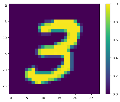
Hiển thị ví dụ đầu tiên:
print(y_train[0])

plt.imshow(x_train[0, :, :, 0])
plt.colorbar()
True
<matplotlib.colorbar.Colorbar at 0x7fac6ad4bd90>
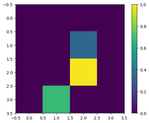
1.2 Giảm tỷ lệ hình ảnh
Kích thước hình ảnh 28x28 là quá lớn đối với các máy tính lượng tử hiện nay. Thay đổi kích thước hình ảnh xuống 4x4:
x_train_small = tf.image.resize(x_train, (4,4)).numpy()
x_test_small = tf.image.resize(x_test, (4,4)).numpy()
Một lần nữa, hãy hiển thị ví dụ đào tạo đầu tiên — sau khi thay đổi kích thước:
print(y_train[0])

plt.imshow(x_train_small[0,:,:,0], vmin=0, vmax=1)
plt.colorbar()
True
<matplotlib.colorbar.Colorbar at 0x7fabf807fe10>
1.3 Loại bỏ các ví dụ mâu thuẫn
Từ phần 3.3 Học cách phân biệt các chữ số của Farhi và cộng sự. , lọc tập dữ liệu để loại bỏ các hình ảnh được gắn nhãn là thuộc cả hai lớp.
Đây không phải là một quy trình học máy tiêu chuẩn, nhưng được đưa vào lợi ích của việc làm theo bài báo.
def remove_contradicting(xs, ys):
    mapping = collections.defaultdict(set)
    orig_x = {}
    # Determine the set of labels for each unique image:
    for x,y in zip(xs,ys):
       orig_x[tuple(x.flatten())] = x
       mapping[tuple(x.flatten())].add(y)

    new_x = []
    new_y = []
    for flatten_x in mapping:
      x = orig_x[flatten_x]
      labels = mapping[flatten_x]
      if len(labels) == 1:
          new_x.append(x)
          new_y.append(next(iter(labels)))
      else:
          # Throw out images that match more than one label.
          pass

    num_uniq_3 = sum(1 for value in mapping.values() if len(value) == 1 and True in value)
    num_uniq_6 = sum(1 for value in mapping.values() if len(value) == 1 and False in value)
    num_uniq_both = sum(1 for value in mapping.values() if len(value) == 2)

    print("Number of unique images:", len(mapping.values()))
    print("Number of unique 3s: ", num_uniq_3)
    print("Number of unique 6s: ", num_uniq_6)
    print("Number of unique contradicting labels (both 3 and 6): ", num_uniq_both)
    print()
    print("Initial number of images: ", len(xs))
    print("Remaining non-contradicting unique images: ", len(new_x))

    return np.array(new_x), np.array(new_y)
Các số lượng kết quả không khớp chặt chẽ với các giá trị được báo cáo, nhưng quy trình chính xác không được chỉ định.
Cũng cần lưu ý ở đây rằng việc áp dụng lọc các ví dụ mâu thuẫn tại thời điểm này không hoàn toàn ngăn cản mô hình nhận các ví dụ huấn luyện mâu thuẫn: bước tiếp theo phân biệt dữ liệu sẽ gây ra nhiều xung đột hơn.
x_train_nocon, y_train_nocon = remove_contradicting(x_train_small, y_train)
Number of unique images: 10387
Number of unique 3s:  4912
Number of unique 6s:  5426
Number of unique contradicting labels (both 3 and 6):  49

Initial number of images:  12049
Remaining non-contradicting unique images:  10338
1.4 Mã hóa dữ liệu dưới dạng mạch lượng tử
Để xử lý hình ảnh bằng máy tính lượng tử, Farhi et al. đề xuất đại diện cho mỗi pixel bằng qubit, với trạng thái tùy thuộc vào giá trị của pixel. Bước đầu tiên là chuyển đổi sang bảng mã nhị phân.
THRESHOLD = 0.5

x_train_bin = np.array(x_train_nocon > THRESHOLD, dtype=np.float32)
x_test_bin = np.array(x_test_small > THRESHOLD, dtype=np.float32)
Nếu bạn loại bỏ những hình ảnh mâu thuẫn vào thời điểm này, bạn sẽ chỉ còn lại 193, có khả năng là không đủ để đào tạo hiệu quả.
_ = remove_contradicting(x_train_bin, y_train_nocon)
Number of unique images: 193
Number of unique 3s:  80
Number of unique 6s:  69
Number of unique contradicting labels (both 3 and 6):  44

Initial number of images:  10338
Remaining non-contradicting unique images:  149
Các qubit tại chỉ số pixel có giá trị vượt quá ngưỡng, được xoay qua cổng \(X\) .
def convert_to_circuit(image):
    """Encode truncated classical image into quantum datapoint."""
    values = np.ndarray.flatten(image)
    qubits = cirq.GridQubit.rect(4, 4)
    circuit = cirq.Circuit()
    for i, value in enumerate(values):
        if value:
            circuit.append(cirq.X(qubits[i]))
    return circuit


x_train_circ = [convert_to_circuit(x) for x in x_train_bin]
x_test_circ = [convert_to_circuit(x) for x in x_test_bin]
Đây là mạch được tạo cho ví dụ đầu tiên (sơ đồ mạch không hiển thị các qubit có cổng 0):
SVGCircuit(x_train_circ[0])
findfont: Font family ['Arial'] not found. Falling back to DejaVu Sans.

So sánh mạch này với các chỉ số mà giá trị hình ảnh vượt quá ngưỡng:
bin_img = x_train_bin[0,:,:,0]
indices = np.array(np.where(bin_img)).T
indices
array([[2, 2],
       [3, 1]])
Chuyển đổi các mạch Cirq này thành tensor cho tfq :
x_train_tfcirc = tfq.convert_to_tensor(x_train_circ)
x_test_tfcirc = tfq.convert_to_tensor(x_test_circ)
2. Mạng nơron lượng tử
Có rất ít hướng dẫn về cấu trúc mạch lượng tử phân loại hình ảnh. Vì sự phân loại dựa trên kỳ vọng của qubit đọc được, Farhi et al. đề xuất sử dụng hai cổng qubit, với qubit đọc ra luôn hoạt động. Điều này tương tự trong một số cách để chạy một RNN đơn nhất nhỏ trên các pixel.
2.1 Xây dựng mạch mô hình
Ví dụ sau đây cho thấy cách tiếp cận phân lớp này. Mỗi lớp sử dụng n phiên bản của cùng một cổng, với mỗi qubit dữ liệu hoạt động trên qubit đọc.
Bắt đầu với một lớp đơn giản sẽ thêm một lớp các cổng này vào mạch:
class CircuitLayerBuilder():
    def __init__(self, data_qubits, readout):
        self.data_qubits = data_qubits
        self.readout = readout

    def add_layer(self, circuit, gate, prefix):
        for i, qubit in enumerate(self.data_qubits):
            symbol = sympy.Symbol(prefix + '-' + str(i))
            circuit.append(gate(qubit, self.readout)**symbol)
Xây dựng một lớp mạch ví dụ để xem nó trông như thế nào:
demo_builder = CircuitLayerBuilder(data_qubits = cirq.GridQubit.rect(4,1),
                                   readout=cirq.GridQubit(-1,-1))

circuit = cirq.Circuit()
demo_builder.add_layer(circuit, gate = cirq.XX, prefix='xx')
SVGCircuit(circuit)

Bây giờ, hãy xây dựng một mô hình hai lớp, phù hợp với kích thước mạch dữ liệu và bao gồm các hoạt động chuẩn bị và đọc.
def create_quantum_model():
    """Create a QNN model circuit and readout operation to go along with it."""
    data_qubits = cirq.GridQubit.rect(4, 4)  # a 4x4 grid.
    readout = cirq.GridQubit(-1, -1)         # a single qubit at [-1,-1]
    circuit = cirq.Circuit()

    # Prepare the readout qubit.
    circuit.append(cirq.X(readout))
    circuit.append(cirq.H(readout))

    builder = CircuitLayerBuilder(
        data_qubits = data_qubits,
        readout=readout)

    # Then add layers (experiment by adding more).
    builder.add_layer(circuit, cirq.XX, "xx1")
    builder.add_layer(circuit, cirq.ZZ, "zz1")

    # Finally, prepare the readout qubit.
    circuit.append(cirq.H(readout))

    return circuit, cirq.Z(readout)
model_circuit, model_readout = create_quantum_model()
2.2 Bọc mạch mô hình trong mô hình tfq-keras
Xây dựng mô hình Keras với các thành phần lượng tử. Mô hình này được cung cấp "dữ liệu lượng tử", từ x_train_circ , mã hóa dữ liệu cổ điển. Nó sử dụng lớp Mạch lượng tử tham số , tfq.layers.PQC , để đào tạo mạch mô hình, trên dữ liệu lượng tử.
Để phân loại những hình ảnh này, Farhi et al. đề xuất lấy kỳ vọng của một qubit đọc trong một mạch tham số hóa. Kỳ vọng trả về giá trị từ 1 đến -1.
# Build the Keras model.
model = tf.keras.Sequential([
    # The input is the data-circuit, encoded as a tf.string
    tf.keras.layers.Input(shape=(), dtype=tf.string),
    # The PQC layer returns the expected value of the readout gate, range [-1,1].
    tfq.layers.PQC(model_circuit, model_readout),
])
Tiếp theo, mô tả thủ tục đào tạo với mô hình, sử dụng phương pháp compile .
Vì mức đọc dự kiến nằm trong khoảng [-1,1] , nên việc tối ưu hóa tổn thất bản lề là một điều phù hợp hơi tự nhiên.
Để sử dụng mất bản lề ở đây bạn cần thực hiện hai điều chỉnh nhỏ. Đầu tiên chuyển đổi các nhãn, y_train_nocon , từ boolean thành [-1,1] , như mong đợi do mất bản lề.
y_train_hinge = 2.0*y_train_nocon-1.0
y_test_hinge = 2.0*y_test-1.0
Thứ hai, sử dụng số liệu hinge_accuracy xử lý chính xác [-1, 1] làm đối số nhãn y_true . tf.losses.BinaryAccuracy(threshold=0.0) mong đợi y_true là boolean và do đó không thể được sử dụng khi mất bản lề).
def hinge_accuracy(y_true, y_pred):
    y_true = tf.squeeze(y_true) > 0.0
    y_pred = tf.squeeze(y_pred) > 0.0
    result = tf.cast(y_true == y_pred, tf.float32)

    return tf.reduce_mean(result)
model.compile(
    loss=tf.keras.losses.Hinge(),
    optimizer=tf.keras.optimizers.Adam(),
    metrics=[hinge_accuracy])
print(model.summary())
Model: "sequential"
_________________________________________________________________
 Layer (type)                Output Shape              Param #
=================================================================
 pqc (PQC)                   (None, 1)                 32

=================================================================
Total params: 32
Trainable params: 32
Non-trainable params: 0
_________________________________________________________________
None
Đào tạo mô hình lượng tử
Bây giờ đào tạo mô hình — quá trình này mất khoảng 45 phút. Nếu bạn không muốn đợi lâu như vậy, hãy sử dụng một tập nhỏ dữ liệu (đặt NUM_EXAMPLES=500 , bên dưới). Điều này không thực sự ảnh hưởng đến tiến trình của mô hình trong quá trình đào tạo (nó chỉ có 32 tham số và không cần nhiều dữ liệu để ràng buộc chúng). Sử dụng ít ví dụ hơn chỉ kết thúc đào tạo sớm hơn (5 phút), nhưng chạy đủ lâu để cho thấy rằng nó đang tiến bộ trong nhật ký xác thực.
EPOCHS = 3
BATCH_SIZE = 32

NUM_EXAMPLES = len(x_train_tfcirc)
x_train_tfcirc_sub = x_train_tfcirc[:NUM_EXAMPLES]
y_train_hinge_sub = y_train_hinge[:NUM_EXAMPLES]
Việc huấn luyện mô hình này đến sự hội tụ cần đạt được độ chính xác> 85% trên bộ thử nghiệm.
qnn_history = model.fit(
      x_train_tfcirc_sub, y_train_hinge_sub,
      batch_size=32,
      epochs=EPOCHS,
      verbose=1,
      validation_data=(x_test_tfcirc, y_test_hinge))

qnn_results = model.evaluate(x_test_tfcirc, y_test)
Epoch 1/3
324/324 [==============================] - 68s 207ms/step - loss: 0.6745 - hinge_accuracy: 0.7719 - val_loss: 0.3959 - val_hinge_accuracy: 0.8004
Epoch 2/3
324/324 [==============================] - 68s 209ms/step - loss: 0.3964 - hinge_accuracy: 0.8291 - val_loss: 0.3498 - val_hinge_accuracy: 0.8997
Epoch 3/3
324/324 [==============================] - 66s 204ms/step - loss: 0.3599 - hinge_accuracy: 0.8854 - val_loss: 0.3395 - val_hinge_accuracy: 0.9042
62/62 [==============================] - 3s 41ms/step - loss: 0.3395 - hinge_accuracy: 0.9042
3. Mạng nơron cổ điển
Trong khi mạng nơ-ron lượng tử hoạt động cho bài toán MNIST đơn giản này, một mạng nơ-ron cổ điển cơ bản có thể dễ dàng làm tốt hơn QNN trong nhiệm vụ này. Sau một kỷ nguyên duy nhất, mạng nơ-ron cổ điển có thể đạt được độ chính xác> 98% trên bộ lưu giữ.
Trong ví dụ sau, một mạng nơ-ron cổ điển được sử dụng cho bài toán phân loại 3-6 bằng cách sử dụng toàn bộ hình ảnh 28x28 thay vì lấy mẫu hình ảnh. Điều này dễ dàng hội tụ đến độ chính xác gần như 100% của bộ thử nghiệm.
def create_classical_model():
    # A simple model based off LeNet from https://keras.io/examples/mnist_cnn/
    model = tf.keras.Sequential()
    model.add(tf.keras.layers.Conv2D(32, [3, 3], activation='relu', input_shape=(28,28,1)))
    model.add(tf.keras.layers.Conv2D(64, [3, 3], activation='relu'))
    model.add(tf.keras.layers.MaxPooling2D(pool_size=(2, 2)))
    model.add(tf.keras.layers.Dropout(0.25))
    model.add(tf.keras.layers.Flatten())
    model.add(tf.keras.layers.Dense(128, activation='relu'))
    model.add(tf.keras.layers.Dropout(0.5))
    model.add(tf.keras.layers.Dense(1))
    return model


model = create_classical_model()
model.compile(loss=tf.keras.losses.BinaryCrossentropy(from_logits=True),
              optimizer=tf.keras.optimizers.Adam(),
              metrics=['accuracy'])

model.summary()
Model: "sequential_1"
_________________________________________________________________
 Layer (type)                Output Shape              Param #
=================================================================
 conv2d (Conv2D)             (None, 26, 26, 32)        320

 conv2d_1 (Conv2D)           (None, 24, 24, 64)        18496

 max_pooling2d (MaxPooling2D  (None, 12, 12, 64)       0
 )

 dropout (Dropout)           (None, 12, 12, 64)        0

 flatten (Flatten)           (None, 9216)              0

 dense (Dense)               (None, 128)               1179776

 dropout_1 (Dropout)         (None, 128)               0

 dense_1 (Dense)             (None, 1)                 129

=================================================================
Total params: 1,198,721
Trainable params: 1,198,721
Non-trainable params: 0
_________________________________________________________________
model.fit(x_train,
          y_train,
          batch_size=128,
          epochs=1,
          verbose=1,
          validation_data=(x_test, y_test))

cnn_results = model.evaluate(x_test, y_test)
95/95 [==============================] - 3s 31ms/step - loss: 0.0400 - accuracy: 0.9842 - val_loss: 0.0057 - val_accuracy: 0.9970
62/62 [==============================] - 0s 3ms/step - loss: 0.0057 - accuracy: 0.9970
Mô hình trên có thông số gần 1,2M. Để so sánh công bằng hơn, hãy thử mô hình 37 tham số, trên các hình ảnh được lấy mẫu con:
def create_fair_classical_model():
    # A simple model based off LeNet from https://keras.io/examples/mnist_cnn/
    model = tf.keras.Sequential()
    model.add(tf.keras.layers.Flatten(input_shape=(4,4,1)))
    model.add(tf.keras.layers.Dense(2, activation='relu'))
    model.add(tf.keras.layers.Dense(1))
    return model


model = create_fair_classical_model()
model.compile(loss=tf.keras.losses.BinaryCrossentropy(from_logits=True),
              optimizer=tf.keras.optimizers.Adam(),
              metrics=['accuracy'])

model.summary()
Model: "sequential_2"
_________________________________________________________________
 Layer (type)                Output Shape              Param #
=================================================================
 flatten_1 (Flatten)         (None, 16)                0

 dense_2 (Dense)             (None, 2)                 34

 dense_3 (Dense)             (None, 1)                 3

=================================================================
Total params: 37
Trainable params: 37
Non-trainable params: 0
_________________________________________________________________
model.fit(x_train_bin,
          y_train_nocon,
          batch_size=128,
          epochs=20,
          verbose=2,
          validation_data=(x_test_bin, y_test))

fair_nn_results = model.evaluate(x_test_bin, y_test)
Epoch 1/20
81/81 - 1s - loss: 0.6678 - accuracy: 0.6546 - val_loss: 0.6326 - val_accuracy: 0.7358 - 503ms/epoch - 6ms/step
Epoch 2/20
81/81 - 0s - loss: 0.6186 - accuracy: 0.7654 - val_loss: 0.5787 - val_accuracy: 0.7515 - 98ms/epoch - 1ms/step
Epoch 3/20
81/81 - 0s - loss: 0.5629 - accuracy: 0.7861 - val_loss: 0.5247 - val_accuracy: 0.7764 - 104ms/epoch - 1ms/step
Epoch 4/20
81/81 - 0s - loss: 0.5150 - accuracy: 0.8301 - val_loss: 0.4825 - val_accuracy: 0.8196 - 103ms/epoch - 1ms/step
Epoch 5/20
81/81 - 0s - loss: 0.4762 - accuracy: 0.8493 - val_loss: 0.4490 - val_accuracy: 0.8293 - 97ms/epoch - 1ms/step
Epoch 6/20
81/81 - 0s - loss: 0.4438 - accuracy: 0.8527 - val_loss: 0.4216 - val_accuracy: 0.8298 - 99ms/epoch - 1ms/step
Epoch 7/20
81/81 - 0s - loss: 0.4169 - accuracy: 0.8555 - val_loss: 0.3986 - val_accuracy: 0.8313 - 98ms/epoch - 1ms/step
Epoch 8/20
81/81 - 0s - loss: 0.3951 - accuracy: 0.8595 - val_loss: 0.3794 - val_accuracy: 0.8313 - 105ms/epoch - 1ms/step
Epoch 9/20
81/81 - 0s - loss: 0.3773 - accuracy: 0.8596 - val_loss: 0.3635 - val_accuracy: 0.8328 - 98ms/epoch - 1ms/step
Epoch 10/20
81/81 - 0s - loss: 0.3620 - accuracy: 0.8611 - val_loss: 0.3499 - val_accuracy: 0.8333 - 97ms/epoch - 1ms/step
Epoch 11/20
81/81 - 0s - loss: 0.3488 - accuracy: 0.8714 - val_loss: 0.3382 - val_accuracy: 0.8720 - 98ms/epoch - 1ms/step
Epoch 12/20
81/81 - 0s - loss: 0.3372 - accuracy: 0.8831 - val_loss: 0.3279 - val_accuracy: 0.8720 - 95ms/epoch - 1ms/step
Epoch 13/20
81/81 - 0s - loss: 0.3271 - accuracy: 0.8831 - val_loss: 0.3187 - val_accuracy: 0.8725 - 97ms/epoch - 1ms/step
Epoch 14/20
81/81 - 0s - loss: 0.3181 - accuracy: 0.8832 - val_loss: 0.3107 - val_accuracy: 0.8725 - 96ms/epoch - 1ms/step
Epoch 15/20
81/81 - 0s - loss: 0.3101 - accuracy: 0.8833 - val_loss: 0.3035 - val_accuracy: 0.8725 - 96ms/epoch - 1ms/step
Epoch 16/20
81/81 - 0s - loss: 0.3030 - accuracy: 0.8833 - val_loss: 0.2972 - val_accuracy: 0.8725 - 105ms/epoch - 1ms/step
Epoch 17/20
81/81 - 0s - loss: 0.2966 - accuracy: 0.8833 - val_loss: 0.2913 - val_accuracy: 0.8725 - 104ms/epoch - 1ms/step
Epoch 18/20
81/81 - 0s - loss: 0.2908 - accuracy: 0.8928 - val_loss: 0.2861 - val_accuracy: 0.8725 - 104ms/epoch - 1ms/step
Epoch 19/20
81/81 - 0s - loss: 0.2856 - accuracy: 0.8955 - val_loss: 0.2816 - val_accuracy: 0.8725 - 99ms/epoch - 1ms/step
Epoch 20/20
81/81 - 0s - loss: 0.2809 - accuracy: 0.8952 - val_loss: 0.2773 - val_accuracy: 0.8725 - 101ms/epoch - 1ms/step
62/62 [==============================] - 0s 895us/step - loss: 0.2773 - accuracy: 0.8725
4. So sánh
Đầu vào có độ phân giải cao hơn và mô hình mạnh mẽ hơn làm cho vấn đề này trở nên dễ dàng với CNN. Trong khi một mô hình cổ điển có công suất tương tự (~ 32 tham số) đào tạo đến độ chính xác tương tự trong một phần nhỏ thời gian. Bằng cách này hay cách khác, mạng nơ-ron cổ điển dễ dàng vượt trội hơn mạng nơ-ron lượng tử. Đối với dữ liệu cổ điển, rất khó để đánh bại mạng nơ-ron cổ điển.
qnn_accuracy = qnn_results[1]
cnn_accuracy = cnn_results[1]
fair_nn_accuracy = fair_nn_results[1]

sns.barplot(["Quantum", "Classical, full", "Classical, fair"],
            [qnn_accuracy, cnn_accuracy, fair_nn_accuracy])
/tmpfs/src/tf_docs_env/lib/python3.7/site-packages/seaborn/_decorators.py:43: FutureWarning: Pass the following variables as keyword args: x, y. From version 0.12, the only valid positional argument will be `data`, and passing other arguments without an explicit keyword will result in an error or misinterpretation.
  FutureWarning
<AxesSubplot:>
