
| | |  Xem nguồn trên GitHub Xem nguồn trên GitHub | |
TensorFlow Quantum đưa các nguyên thủy lượng tử vào hệ sinh thái TensorFlow. Giờ đây, các nhà nghiên cứu lượng tử có thể tận dụng các công cụ từ TensorFlow. Trong hướng dẫn này, bạn sẽ xem xét kỹ hơn việc kết hợp TensorBoard vào nghiên cứu điện toán lượng tử của mình. Sử dụng hướng dẫn DCGAN từ TensorFlow, bạn sẽ nhanh chóng xây dựng các thử nghiệm và hình ảnh hóa làm việc tương tự như các thử nghiệm được thực hiện bởi Niu et al. . Nói rộng ra bạn sẽ:
- Đào tạo GAN để tạo ra các mẫu trông giống như chúng đến từ các mạch lượng tử.
- Hình dung quá trình đào tạo cũng như sự phát triển của phân phối theo thời gian.
- Đánh giá thử nghiệm bằng cách khám phá biểu đồ tính toán.
pip install tensorflow==2.7.0 tensorflow-quantum tensorboard_plugin_profile==2.4.0
# Update package resources to account for version changes.
import importlib, pkg_resources
importlib.reload(pkg_resources)
<module 'pkg_resources' from '/tmpfs/src/tf_docs_env/lib/python3.7/site-packages/pkg_resources/__init__.py'>
#docs_infra: no_execute
%load_ext tensorboard
import datetime
import time
import cirq
import tensorflow as tf
import tensorflow_quantum as tfq
from tensorflow.keras import layers

# visualization tools
%matplotlib inline
import matplotlib.pyplot as plt
from cirq.contrib.svg import SVGCircuit
2022-02-04 12:46:52.770534: E tensorflow/stream_executor/cuda/cuda_driver.cc:271] failed call to cuInit: CUDA_ERROR_NO_DEVICE: no CUDA-capable device is detected
1. Tạo dữ liệu
Bắt đầu bằng cách thu thập một số dữ liệu. Bạn có thể sử dụng TensorFlow Quantum để nhanh chóng tạo một số mẫu chuỗi bit sẽ là nguồn dữ liệu chính cho phần còn lại của các thử nghiệm của bạn. Giống như Niu et al. bạn sẽ khám phá việc mô phỏng lấy mẫu từ các mạch ngẫu nhiên dễ dàng như thế nào với độ sâu giảm đáng kể. Đầu tiên, hãy xác định một số trình trợ giúp:
def generate_circuit(qubits):
    """Generate a random circuit on qubits."""
    random_circuit = cirq.generate_boixo_2018_supremacy_circuits_v2(
        qubits, cz_depth=2, seed=1234)
    return random_circuit

def generate_data(circuit, n_samples):
    """Draw n_samples samples from circuit into a tf.Tensor."""
    return tf.squeeze(tfq.layers.Sample()(circuit, repetitions=n_samples).to_tensor())
Bây giờ bạn có thể kiểm tra mạch cũng như một số dữ liệu mẫu:
qubits = cirq.GridQubit.rect(1, 5)
random_circuit_m = generate_circuit(qubits) + cirq.measure_each(*qubits)
SVGCircuit(random_circuit_m)
findfont: Font family ['Arial'] not found. Falling back to DejaVu Sans.

samples = cirq.sample(random_circuit_m, repetitions=10)
print('10 Random bitstrings from this circuit:')
print(samples)
10 Random bitstrings from this circuit:
(0, 0)=1000001000
(0, 1)=0000001010
(0, 2)=1010000100
(0, 3)=0010000110
(0, 4)=0110110010
Bạn có thể làm điều tương tự trong TensorFlow Quantum với:
generate_data(random_circuit_m, 10)
<tf.Tensor: shape=(10, 5), dtype=int8, numpy=
array([[0, 0, 0, 0, 0],
       [0, 0, 0, 0, 0],
       [0, 0, 1, 0, 0],
       [0, 1, 0, 0, 0],
       [0, 1, 0, 0, 0],
       [0, 1, 1, 0, 0],
       [1, 0, 0, 0, 0],
       [1, 0, 0, 1, 0],
       [1, 1, 1, 0, 0],
       [1, 1, 1, 0, 0]], dtype=int8)>
Giờ đây, bạn có thể nhanh chóng tạo dữ liệu đào tạo của mình bằng:
N_SAMPLES = 60000
N_QUBITS = 10
QUBITS = cirq.GridQubit.rect(1, N_QUBITS)
REFERENCE_CIRCUIT = generate_circuit(QUBITS)
all_data = generate_data(REFERENCE_CIRCUIT, N_SAMPLES)
all_data
<tf.Tensor: shape=(60000, 10), dtype=int8, numpy=
array([[0, 0, 0, ..., 0, 0, 0],
       [0, 0, 0, ..., 0, 0, 0],
       [0, 0, 0, ..., 0, 0, 0],
       ...,
       [1, 1, 1, ..., 1, 1, 1],
       [1, 1, 1, ..., 1, 1, 1],
       [1, 1, 1, ..., 1, 1, 1]], dtype=int8)>
Sẽ rất hữu ích khi xác định một số chức năng trợ giúp để hình dung khi quá trình đào tạo được tiến hành. Hai đại lượng thú vị để sử dụng là:
- Giá trị nguyên của các mẫu để bạn có thể tạo biểu đồ của phân phối.
- Ước tính độ trung thực XEB tuyến tính của một tập hợp các mẫu, để đưa ra một số dấu hiệu về mức độ "thực sự ngẫu nhiên lượng tử" của các mẫu.
@tf.function
def bits_to_ints(bits):
    """Convert tensor of bitstrings to tensor of ints."""
    sigs = tf.constant([1 << i for i in range(N_QUBITS)], dtype=tf.int32)
    rounded_bits = tf.clip_by_value(tf.math.round(
        tf.cast(bits, dtype=tf.dtypes.float32)), clip_value_min=0, clip_value_max=1)
    return tf.einsum('jk,k->j', tf.cast(rounded_bits, dtype=tf.dtypes.int32), sigs)

@tf.function
def xeb_fid(bits):
    """Compute linear XEB fidelity of bitstrings."""
    final_probs = tf.squeeze(
        tf.abs(tfq.layers.State()(REFERENCE_CIRCUIT).to_tensor()) ** 2)
    nums = bits_to_ints(bits)
    return (2 ** N_QUBITS) * tf.reduce_mean(tf.gather(final_probs, nums)) - 1.0
Tại đây, bạn có thể hình dung sự phân phối và kiểm tra sự tỉnh táo của mình bằng XEB:
plt.hist(bits_to_ints(all_data).numpy(), 50)
plt.show()
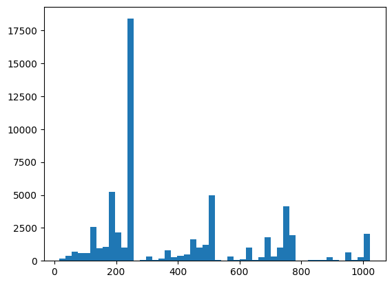
xeb_fid(all_data)
<tf.Tensor: shape=(), dtype=float32, numpy=-0.0015467405>
2. Xây dựng mô hình
Tại đây, bạn có thể sử dụng các thành phần liên quan từ hướng dẫn DCGAN cho trường hợp lượng tử. Thay vì tạo ra các chữ số MNIST, GAN mới sẽ được sử dụng để tạo ra các mẫu chuỗi bit có độ dài N_QUBITS
LATENT_DIM = 100
def make_generator_model():
    """Construct generator model."""
    model = tf.keras.Sequential()
    model.add(layers.Dense(256, use_bias=False, input_shape=(LATENT_DIM,)))
    model.add(layers.Dense(128, activation='relu'))
    model.add(layers.Dropout(0.3))
    model.add(layers.Dense(64, activation='relu'))
    model.add(layers.Dense(N_QUBITS, activation='relu'))

    return model

def make_discriminator_model():
    """Constrcut discriminator model."""
    model = tf.keras.Sequential()
    model.add(layers.Dense(256, use_bias=False, input_shape=(N_QUBITS,)))
    model.add(layers.Dense(128, activation='relu'))
    model.add(layers.Dropout(0.3))
    model.add(layers.Dense(32, activation='relu'))
    model.add(layers.Dense(1))

    return model
Tiếp theo, khởi tạo mô hình trình tạo và mô hình phân biệt, xác định tổn thất và tạo hàm train_step để sử dụng cho vòng lặp đào tạo chính của bạn:
discriminator = make_discriminator_model()
generator = make_generator_model()
cross_entropy = tf.keras.losses.BinaryCrossentropy(from_logits=True)
def discriminator_loss(real_output, fake_output):
    """Compute discriminator loss."""
    real_loss = cross_entropy(tf.ones_like(real_output), real_output)
    fake_loss = cross_entropy(tf.zeros_like(fake_output), fake_output)
    total_loss = real_loss + fake_loss
    return total_loss

def generator_loss(fake_output):
    """Compute generator loss."""
    return cross_entropy(tf.ones_like(fake_output), fake_output)

generator_optimizer = tf.keras.optimizers.Adam(1e-4)
discriminator_optimizer = tf.keras.optimizers.Adam(1e-4)
BATCH_SIZE=256

@tf.function
def train_step(images):
    """Run train step on provided image batch."""
    noise = tf.random.normal([BATCH_SIZE, LATENT_DIM])
    with tf.GradientTape() as gen_tape, tf.GradientTape() as disc_tape:
        generated_images = generator(noise, training=True)

        real_output = discriminator(images, training=True)
        fake_output = discriminator(generated_images, training=True)

        gen_loss = generator_loss(fake_output)
        disc_loss = discriminator_loss(real_output, fake_output)

    gradients_of_generator = gen_tape.gradient(
        gen_loss, generator.trainable_variables)
    gradients_of_discriminator = disc_tape.gradient(
        disc_loss, discriminator.trainable_variables)

    generator_optimizer.apply_gradients(
        zip(gradients_of_generator, generator.trainable_variables))
    discriminator_optimizer.apply_gradients(
        zip(gradients_of_discriminator, discriminator.trainable_variables))

    return gen_loss, disc_loss
Bây giờ bạn đã có tất cả các khối xây dựng cần thiết cho mô hình của mình, bạn có thể thiết lập một chức năng đào tạo kết hợp trực quan hóa TensorBoard. Đầu tiên thiết lập trình ghi tệp TensorBoard:
logdir = "tb_logs/" + datetime.datetime.now().strftime("%Y%m%d-%H%M%S")
file_writer = tf.summary.create_file_writer(logdir + "/metrics")
file_writer.set_as_default()
Sử dụng mô-đun tf.summary , giờ đây bạn có thể kết hợp ghi nhật ký scalar , histogram (cũng như các biểu đồ khác) vào TensorBoard bên trong chức năng train chính:
def train(dataset, epochs, start_epoch=1):
    """Launch full training run for the given number of epochs."""
    # Log original training distribution.
    tf.summary.histogram('Training Distribution', data=bits_to_ints(dataset), step=0)

    batched_data = tf.data.Dataset.from_tensor_slices(dataset).shuffle(N_SAMPLES).batch(512)
    t = time.time()
    for epoch in range(start_epoch, start_epoch + epochs):
        for i, image_batch in enumerate(batched_data):
            # Log batch-wise loss.
            gl, dl = train_step(image_batch)
            tf.summary.scalar(
                'Generator loss', data=gl, step=epoch * len(batched_data) + i)
            tf.summary.scalar(
                'Discriminator loss', data=dl, step=epoch * len(batched_data) + i)

        # Log full dataset XEB Fidelity and generated distribution.
        generated_samples = generator(tf.random.normal([N_SAMPLES, 100]))
        tf.summary.scalar(
        'Generator XEB Fidelity Estimate', data=xeb_fid(generated_samples), step=epoch)
        tf.summary.histogram(
        'Generator distribution', data=bits_to_ints(generated_samples), step=epoch)
        # Log new samples drawn from this particular random circuit.
        random_new_distribution = generate_data(REFERENCE_CIRCUIT, N_SAMPLES)
        tf.summary.histogram(
        'New round of True samples', data=bits_to_ints(random_new_distribution), step=epoch)

        if epoch % 10 == 0:
            print('Epoch {}, took {}(s)'.format(epoch, time.time() - t))
            t = time.time()
3. Vizualize đào tạo và hiệu suất
Bảng điều khiển TensorBoard hiện có thể được khởi chạy với:
#docs_infra: no_execute
%tensorboard --logdir tb_logs/
Khi gọi train , bảng điều khiển TensoBoard sẽ tự động cập nhật với tất cả các thống kê tóm tắt được cung cấp trong vòng huấn luyện.
train(all_data, epochs=50)
Epoch 10, took 9.325464487075806(s)
Epoch 20, took 7.684147119522095(s)
Epoch 30, took 7.508770704269409(s)
Epoch 40, took 7.5157341957092285(s)
Epoch 50, took 7.533370494842529(s)
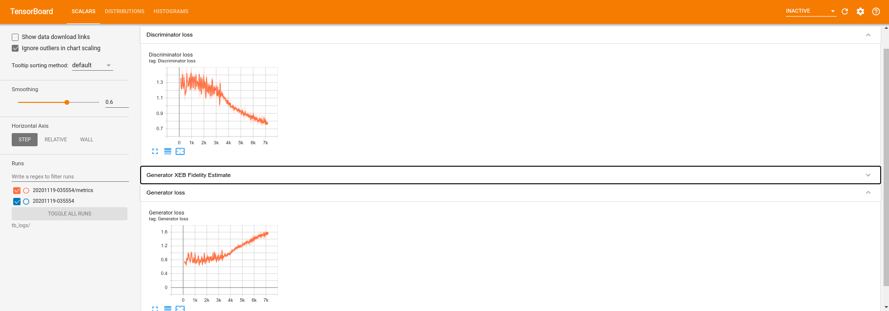
Trong khi quá trình đào tạo đang diễn ra (và sau khi hoàn tất), bạn có thể kiểm tra các đại lượng vô hướng:
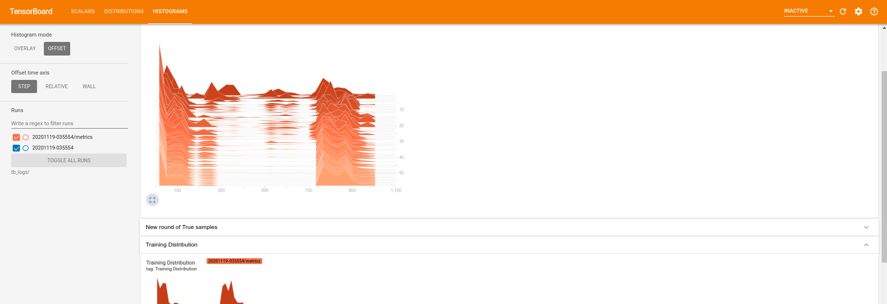
Chuyển sang tab biểu đồ, bạn cũng có thể xem mạng trình tạo hoạt động tốt như thế nào trong việc tạo lại các mẫu từ phân phối lượng tử:
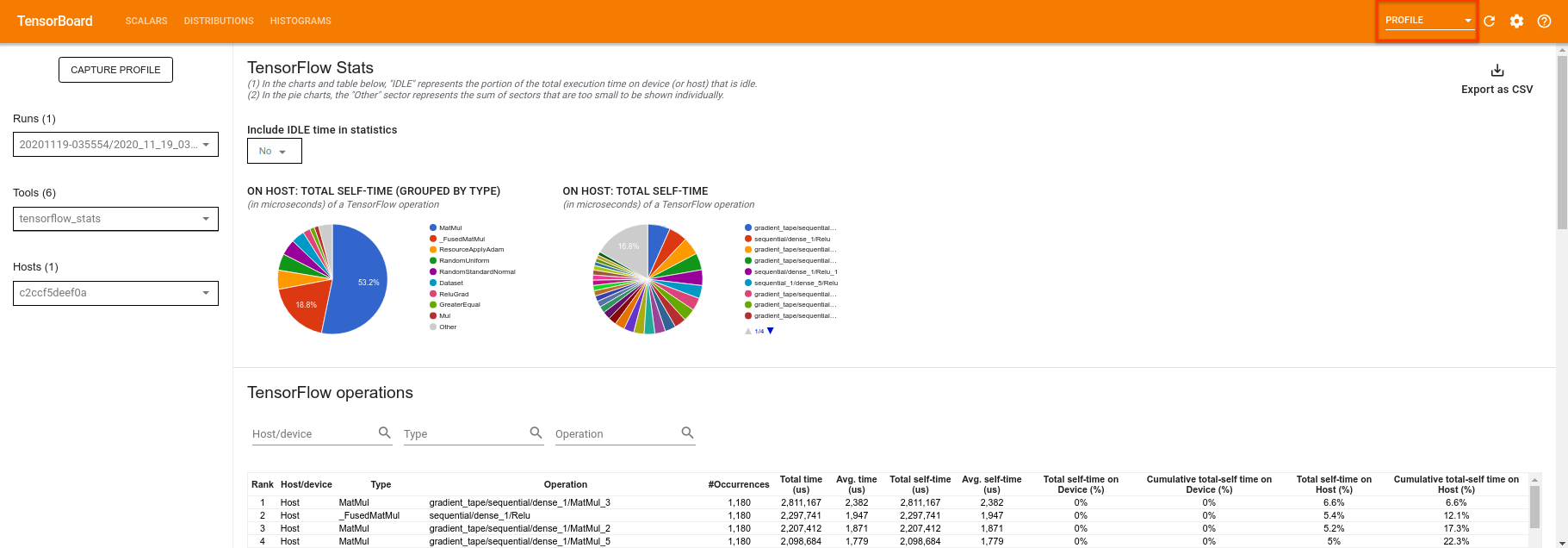
Ngoài việc cho phép theo dõi thời gian thực các thống kê tóm tắt liên quan đến thử nghiệm của bạn, TensorBoard cũng có thể giúp bạn lập hồ sơ các thử nghiệm của mình để xác định các tắc nghẽn về hiệu suất. Để chạy lại mô hình của bạn với giám sát hiệu suất, bạn có thể làm:
tf.profiler.experimental.start(logdir)
train(all_data, epochs=10, start_epoch=50)
tf.profiler.experimental.stop()
Epoch 50, took 0.8879530429840088(s)
TensorBoard sẽ lập hồ sơ tất cả mã giữa tf.profiler.experimental.start và tf.profiler.experimental.stop . Dữ liệu hồ sơ này sau đó có thể được xem trong trang profile của TensorBoard:
Hãy thử tăng độ sâu hoặc thử nghiệm với các lớp mạch lượng tử khác nhau. Kiểm tra tất cả các tính năng tuyệt vời khác của TensorBoard như điều chỉnh siêu thông số mà bạn có thể kết hợp vào các thử nghiệm Lượng tử TensorFlow của mình.