
| |
|
 GitHub でソースを表示 GitHub でソースを表示
|
|
このチュートリアルでは、pandas DataFrames を TensorFlow に読み込む方法の例を示します。
このチュートリアルでは、UCI Machine Learning Repository が提供する小さな心臓疾患データセットを使用します。CSV 形式で数百の行を含むデータセットです。各行は患者に関する情報で、列には属性が記述されています。この情報を使って、患者に心臓疾患があるかどうかを予測します。これは二項分類のタスクです。
pandas を使ってデータを読み取る
import pandas as pd
import tensorflow as tf

SHUFFLE_BUFFER = 500
BATCH_SIZE = 2
2022-12-15 00:56:39.676822: W tensorflow/compiler/xla/stream_executor/platform/default/dso_loader.cc:64] Could not load dynamic library 'libnvinfer.so.7'; dlerror: libnvinfer.so.7: cannot open shared object file: No such file or directory
2022-12-15 00:56:39.676949: W tensorflow/compiler/xla/stream_executor/platform/default/dso_loader.cc:64] Could not load dynamic library 'libnvinfer_plugin.so.7'; dlerror: libnvinfer_plugin.so.7: cannot open shared object file: No such file or directory
2022-12-15 00:56:39.676959: W tensorflow/compiler/tf2tensorrt/utils/py_utils.cc:38] TF-TRT Warning: Cannot dlopen some TensorRT libraries. If you would like to use Nvidia GPU with TensorRT, please make sure the missing libraries mentioned above are installed properly.
心臓疾患データセットを含む CSV ファイルをダウンロードします。
csv_file = tf.keras.utils.get_file('heart.csv', 'https://storage.googleapis.com/download.tensorflow.org/data/heart.csv')
Downloading data from https://storage.googleapis.com/download.tensorflow.org/data/heart.csv
13273/13273 [==============================] - 0s 0us/step
pandas を使って CSV を読み取ります。
df = pd.read_csv(csv_file)
データは以下のように表示されます。
df.head()
df.dtypes
age           int64
sex           int64
cp            int64
trestbps      int64
chol          int64
fbs           int64
restecg       int64
thalach       int64
exang         int64
oldpeak     float64
slope         int64
ca            int64
thal         object
target        int64
dtype: object
target 列に含まれるラベルを予測するモデルを作成します。
target = df.pop('target')
配列としての DataFrame
データのデータ型が統一されている場合、または、dtype の場合、NumPy 配列を使用できる場合であればどこでも pandas DataFrame を使用できます。これは、pandas.DataFrame クラスが __array__ プロトコルをサポートしているためであり、TensorFlow の tf.convert_to_tensor 関数がプロトコルをサポートするオブジェクトを受け入れるます。
データセットから数値特徴量を取得します (ここでは、カテゴリカル特徴量をスキップします)。
numeric_feature_names = ['age', 'thalach', 'trestbps',  'chol', 'oldpeak']
numeric_features = df[numeric_feature_names]
numeric_features.head()
DataFrame は、DataFrame.values プロパティまたは numpy.array(df) を使用して NumPy 配列に変換できます。テンソルに変換するには、tf.convert_to_tensor を使用します。
tf.convert_to_tensor(numeric_features)
<tf.Tensor: shape=(303, 5), dtype=float64, numpy=
array([[ 63. , 150. , 145. , 233. ,   2.3],
       [ 67. , 108. , 160. , 286. ,   1.5],
       [ 67. , 129. , 120. , 229. ,   2.6],
       ...,
       [ 65. , 127. , 135. , 254. ,   2.8],
       [ 48. , 150. , 130. , 256. ,   0. ],
       [ 63. , 154. , 150. , 407. ,   4. ]])>
一般に、オブジェクトを tf.convert_to_tensor でテンソルに変換すれば、tf.Tensor を渡せる場合は、同様に渡すことができます。
Model.fit メソッド
単一のテンソルとして解釈される DataFrame は、Model.fit メソッドの引数として直接使用できます。
以下は、データセットの数値特徴に関するモデルのトレーニングの例です。
最初のステップは、入力範囲を正規化することです。そのために tf.keras.layers.Normalization レイヤーを使用します。
実行する前にレイヤーの平均と標準偏差を設定するには、必ず Normalization.adapt メソッドを呼び出してください。
normalizer = tf.keras.layers.Normalization(axis=-1)
normalizer.adapt(numeric_features)
DataFrame の最初の 3 行でレイヤーを呼び出して、このレイヤーからの出力のサンプルを視覚化します。
normalizer(numeric_features.iloc[:3])
<tf.Tensor: shape=(3, 5), dtype=float32, numpy=
array([[ 0.93383914,  0.03480718,  0.74578077, -0.26008663,  1.0680453 ],
       [ 1.3782105 , -1.7806165 ,  1.5923285 ,  0.7573877 ,  0.38022864],
       [ 1.3782105 , -0.87290466, -0.6651321 , -0.33687714,  1.3259765 ]],
      dtype=float32)>
単純なモデルの最初のレイヤーとして正規化レイヤーを使用します。
def get_basic_model():
  model = tf.keras.Sequential([
    normalizer,
    tf.keras.layers.Dense(10, activation='relu'),
    tf.keras.layers.Dense(10, activation='relu'),
    tf.keras.layers.Dense(1)
  ])

  model.compile(optimizer='adam',
                loss=tf.keras.losses.BinaryCrossentropy(from_logits=True),
                metrics=['accuracy'])
  return model
DataFrame を x 引数として Model.fit に渡すと、Keras は DataFrame をNumPy 配列と同じように扱います。
model = get_basic_model()
model.fit(numeric_features, target, epochs=15, batch_size=BATCH_SIZE)
Epoch 1/15
152/152 [==============================] - 2s 3ms/step - loss: 0.6602 - accuracy: 0.7261
Epoch 2/15
152/152 [==============================] - 0s 3ms/step - loss: 0.5958 - accuracy: 0.7327
Epoch 3/15
152/152 [==============================] - 0s 3ms/step - loss: 0.5444 - accuracy: 0.7393
Epoch 4/15
152/152 [==============================] - 0s 3ms/step - loss: 0.5065 - accuracy: 0.7459
Epoch 5/15
152/152 [==============================] - 0s 3ms/step - loss: 0.4829 - accuracy: 0.7657
Epoch 6/15
152/152 [==============================] - 0s 3ms/step - loss: 0.4678 - accuracy: 0.7690
Epoch 7/15
152/152 [==============================] - 0s 3ms/step - loss: 0.4605 - accuracy: 0.7756
Epoch 8/15
152/152 [==============================] - 0s 3ms/step - loss: 0.4534 - accuracy: 0.7789
Epoch 9/15
152/152 [==============================] - 0s 3ms/step - loss: 0.4465 - accuracy: 0.7822
Epoch 10/15
152/152 [==============================] - 0s 3ms/step - loss: 0.4437 - accuracy: 0.7822
Epoch 11/15
152/152 [==============================] - 0s 3ms/step - loss: 0.4407 - accuracy: 0.7855
Epoch 12/15
152/152 [==============================] - 0s 3ms/step - loss: 0.4360 - accuracy: 0.7921
Epoch 13/15
152/152 [==============================] - 0s 3ms/step - loss: 0.4349 - accuracy: 0.7987
Epoch 14/15
152/152 [==============================] - 0s 3ms/step - loss: 0.4316 - accuracy: 0.7954
Epoch 15/15
152/152 [==============================] - 0s 3ms/step - loss: 0.4305 - accuracy: 0.7987
<keras.callbacks.History at 0x7f07d05e8b80>
tf.data を適用する
tf.data 変換を均一な dtype の DataFrame に適用する場合、Dataset.from_tensor_slices メソッドは、DataFrame の行を反復処理するデータセットを作成します。各行は、最初は値のベクトルです。モデルをトレーニングするには、(inputs, labels) のペアが必要なので、(features, labels) と Dataset.from_tensor_slices を渡し、必要なスライスのペアを取得します。
numeric_dataset = tf.data.Dataset.from_tensor_slices((numeric_features, target))

for row in numeric_dataset.take(3):
  print(row)
(<tf.Tensor: shape=(5,), dtype=float64, numpy=array([ 63. , 150. , 145. , 233. ,   2.3])>, <tf.Tensor: shape=(), dtype=int64, numpy=0>)
(<tf.Tensor: shape=(5,), dtype=float64, numpy=array([ 67. , 108. , 160. , 286. ,   1.5])>, <tf.Tensor: shape=(), dtype=int64, numpy=1>)
(<tf.Tensor: shape=(5,), dtype=float64, numpy=array([ 67. , 129. , 120. , 229. ,   2.6])>, <tf.Tensor: shape=(), dtype=int64, numpy=0>)
numeric_batches = numeric_dataset.shuffle(1000).batch(BATCH_SIZE)

model = get_basic_model()
model.fit(numeric_batches, epochs=15)
Epoch 1/15
152/152 [==============================] - 1s 3ms/step - loss: 0.6889 - accuracy: 0.7327
Epoch 2/15
152/152 [==============================] - 0s 3ms/step - loss: 0.5900 - accuracy: 0.7360
Epoch 3/15
152/152 [==============================] - 0s 3ms/step - loss: 0.5110 - accuracy: 0.7492
Epoch 4/15
152/152 [==============================] - 0s 3ms/step - loss: 0.4667 - accuracy: 0.7591
Epoch 5/15
152/152 [==============================] - 0s 3ms/step - loss: 0.4497 - accuracy: 0.7723
Epoch 6/15
152/152 [==============================] - 0s 3ms/step - loss: 0.4401 - accuracy: 0.7723
Epoch 7/15
152/152 [==============================] - 0s 3ms/step - loss: 0.4346 - accuracy: 0.7723
Epoch 8/15
152/152 [==============================] - 0s 3ms/step - loss: 0.4315 - accuracy: 0.7756
Epoch 9/15
152/152 [==============================] - 0s 3ms/step - loss: 0.4310 - accuracy: 0.7822
Epoch 10/15
152/152 [==============================] - 0s 3ms/step - loss: 0.4271 - accuracy: 0.7888
Epoch 11/15
152/152 [==============================] - 0s 3ms/step - loss: 0.4249 - accuracy: 0.7888
Epoch 12/15
152/152 [==============================] - 0s 3ms/step - loss: 0.4242 - accuracy: 0.7822
Epoch 13/15
152/152 [==============================] - 0s 3ms/step - loss: 0.4209 - accuracy: 0.7987
Epoch 14/15
152/152 [==============================] - 0s 3ms/step - loss: 0.4201 - accuracy: 0.7921
Epoch 15/15
152/152 [==============================] - 0s 3ms/step - loss: 0.4205 - accuracy: 0.7954
<keras.callbacks.History at 0x7f07d0361700>
ディレクトリとしての DataFrame
型が異なるデータを処理する場合、DataFrame を単一の配列であるかのように扱うことができなくなります。TensorFlow テンソルでは、すべての要素が同じ dtype である必要があります。
したがって、この場合、各列が均一な dtype を持つ列のディクショナリとして扱う必要があります。DataFrame は配列のディクショナリによく似ているため、通常、必要なのは DataFrame を Python dict にキャストするだけです。多くの重要な TensorFlow API は、配列の (ネストされた) ディクショナリを入力としてサポートしています。
tf.data 入力パイプラインはこれを非常にうまく処理します。すべての tf.data 演算は、ディクショナリとタプルを自動的に処理するので、DataFrame からディクショナリのサンプルのデータセットを作成するには、Dataset.from_tensor_slices でスライスする前に、それをディクショナリにキャストするだけです。
numeric_dict_ds = tf.data.Dataset.from_tensor_slices((dict(numeric_features), target))
以下はデータセットの最初の 3 つのサンプルです。
for row in numeric_dict_ds.take(3):
  print(row)
({'age': <tf.Tensor: shape=(), dtype=int64, numpy=63>, 'thalach': <tf.Tensor: shape=(), dtype=int64, numpy=150>, 'trestbps': <tf.Tensor: shape=(), dtype=int64, numpy=145>, 'chol': <tf.Tensor: shape=(), dtype=int64, numpy=233>, 'oldpeak': <tf.Tensor: shape=(), dtype=float64, numpy=2.3>}, <tf.Tensor: shape=(), dtype=int64, numpy=0>)
({'age': <tf.Tensor: shape=(), dtype=int64, numpy=67>, 'thalach': <tf.Tensor: shape=(), dtype=int64, numpy=108>, 'trestbps': <tf.Tensor: shape=(), dtype=int64, numpy=160>, 'chol': <tf.Tensor: shape=(), dtype=int64, numpy=286>, 'oldpeak': <tf.Tensor: shape=(), dtype=float64, numpy=1.5>}, <tf.Tensor: shape=(), dtype=int64, numpy=1>)
({'age': <tf.Tensor: shape=(), dtype=int64, numpy=67>, 'thalach': <tf.Tensor: shape=(), dtype=int64, numpy=129>, 'trestbps': <tf.Tensor: shape=(), dtype=int64, numpy=120>, 'chol': <tf.Tensor: shape=(), dtype=int64, numpy=229>, 'oldpeak': <tf.Tensor: shape=(), dtype=float64, numpy=2.6>}, <tf.Tensor: shape=(), dtype=int64, numpy=0>)
Keras のディクショナリ
通常、Keras モデルとレイヤーは単一の入力テンソルを期待しますが、これらのクラスはディクショナリ、タプル、テンソルのネストされた構造を受け入れて返すことができます。これらの構造は「ネスト」と呼ばれます (詳細については、tf.nest モジュールを参照してください)。
ディクショナリを入力として受け入れる Keras モデルを作成するには、2 つの同等の方法があります。
1. モデルサブクラススタイル
tf.keras.Model (または tf.keras.Layer) のサブクラスを記述します。入力を直接処理し、出力を作成します。
def stack_dict(inputs, fun=tf.stack):
    values = []
    for key in sorted(inputs.keys()):
      values.append(tf.cast(inputs[key], tf.float32))

    return fun(values, axis=-1)
class MyModel(tf.keras.Model):
  def __init__(self):
    # Create all the internal layers in init.
    super().__init__(self)

    self.normalizer = tf.keras.layers.Normalization(axis=-1)

    self.seq = tf.keras.Sequential([
      self.normalizer,
      tf.keras.layers.Dense(10, activation='relu'),
      tf.keras.layers.Dense(10, activation='relu'),
      tf.keras.layers.Dense(1)
    ])

  def adapt(self, inputs):
    # Stack the inputs and `adapt` the normalization layer.
    inputs = stack_dict(inputs)
    self.normalizer.adapt(inputs)

  def call(self, inputs):
    # Stack the inputs
    inputs = stack_dict(inputs)
    # Run them through all the layers.
    result = self.seq(inputs)

    return result

model = MyModel()

model.adapt(dict(numeric_features))

model.compile(optimizer='adam',
              loss=tf.keras.losses.BinaryCrossentropy(from_logits=True),
              metrics=['accuracy'],
              run_eagerly=True)
このモデルは、トレーニング用の列のディクショナリまたはディクショナリ要素のデータセットのいずれかを受け入れることができます。
model.fit(dict(numeric_features), target, epochs=5, batch_size=BATCH_SIZE)
Epoch 1/5
WARNING:tensorflow:5 out of the last 5 calls to <function _BaseOptimizer._update_step_xla at 0x7f07d0115280> triggered tf.function retracing. Tracing is expensive and the excessive number of tracings could be due to (1) creating @tf.function repeatedly in a loop, (2) passing tensors with different shapes, (3) passing Python objects instead of tensors. For (1), please define your @tf.function outside of the loop. For (2), @tf.function has reduce_retracing=True option that can avoid unnecessary retracing. For (3), please refer to https://www.tensorflow.org/guide/function#controlling_retracing and https://www.tensorflow.org/api_docs/python/tf/function for  more details.
WARNING:tensorflow:6 out of the last 6 calls to <function _BaseOptimizer._update_step_xla at 0x7f07d0115280> triggered tf.function retracing. Tracing is expensive and the excessive number of tracings could be due to (1) creating @tf.function repeatedly in a loop, (2) passing tensors with different shapes, (3) passing Python objects instead of tensors. For (1), please define your @tf.function outside of the loop. For (2), @tf.function has reduce_retracing=True option that can avoid unnecessary retracing. For (3), please refer to https://www.tensorflow.org/guide/function#controlling_retracing and https://www.tensorflow.org/api_docs/python/tf/function for  more details.
152/152 [==============================] - 4s 25ms/step - loss: 0.7211 - accuracy: 0.7162
Epoch 2/5
152/152 [==============================] - 4s 24ms/step - loss: 0.6226 - accuracy: 0.7261
Epoch 3/5
152/152 [==============================] - 4s 25ms/step - loss: 0.5648 - accuracy: 0.7459
Epoch 4/5
152/152 [==============================] - 4s 24ms/step - loss: 0.5226 - accuracy: 0.7624
Epoch 5/5
152/152 [==============================] - 4s 24ms/step - loss: 0.4927 - accuracy: 0.7789
<keras.callbacks.History at 0x7f07d01f8b80>
numeric_dict_batches = numeric_dict_ds.shuffle(SHUFFLE_BUFFER).batch(BATCH_SIZE)
model.fit(numeric_dict_batches, epochs=5)
Epoch 1/5
152/152 [==============================] - 3s 21ms/step - loss: 0.4750 - accuracy: 0.7756
Epoch 2/5
152/152 [==============================] - 3s 21ms/step - loss: 0.4608 - accuracy: 0.7789
Epoch 3/5
152/152 [==============================] - 3s 21ms/step - loss: 0.4515 - accuracy: 0.7855
Epoch 4/5
152/152 [==============================] - 3s 21ms/step - loss: 0.4427 - accuracy: 0.7789
Epoch 5/5
152/152 [==============================] - 3s 21ms/step - loss: 0.4382 - accuracy: 0.7789
<keras.callbacks.History at 0x7f07d0051160>
最初の 3 つのサンプルの予測は次のとおりです。
model.predict(dict(numeric_features.iloc[:3]))
1/1 [==============================] - 0s 35ms/step
array([[[0.49147445]],

       [[0.5728407 ]],

       [[0.28431088]]], dtype=float32)
2. Keras 関数型スタイル
inputs = {}
for name, column in numeric_features.items():
  inputs[name] = tf.keras.Input(
      shape=(1,), name=name, dtype=tf.float32)

inputs
{'age': <KerasTensor: shape=(None, 1) dtype=float32 (created by layer 'age')>,
 'thalach': <KerasTensor: shape=(None, 1) dtype=float32 (created by layer 'thalach')>,
 'trestbps': <KerasTensor: shape=(None, 1) dtype=float32 (created by layer 'trestbps')>,
 'chol': <KerasTensor: shape=(None, 1) dtype=float32 (created by layer 'chol')>,
 'oldpeak': <KerasTensor: shape=(None, 1) dtype=float32 (created by layer 'oldpeak')>}
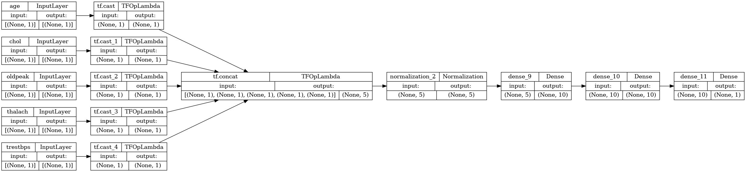
x = stack_dict(inputs, fun=tf.concat)

normalizer = tf.keras.layers.Normalization(axis=-1)
normalizer.adapt(stack_dict(dict(numeric_features)))

x = normalizer(x)
x = tf.keras.layers.Dense(10, activation='relu')(x)
x = tf.keras.layers.Dense(10, activation='relu')(x)
x = tf.keras.layers.Dense(1)(x)

model = tf.keras.Model(inputs, x)

model.compile(optimizer='adam',
              loss=tf.keras.losses.BinaryCrossentropy(from_logits=True),
              metrics=['accuracy'],
              run_eagerly=True)
tf.keras.utils.plot_model(model, rankdir="LR", show_shapes=True)
モデルサブクラスと同じ方法で関数モデルをトレーニングできます。
model.fit(dict(numeric_features), target, epochs=5, batch_size=BATCH_SIZE)
Epoch 1/5
152/152 [==============================] - 4s 23ms/step - loss: 0.7955 - accuracy: 0.6073
Epoch 2/5
152/152 [==============================] - 3s 22ms/step - loss: 0.6508 - accuracy: 0.7360
Epoch 3/5
152/152 [==============================] - 3s 22ms/step - loss: 0.5798 - accuracy: 0.7360
Epoch 4/5
152/152 [==============================] - 3s 21ms/step - loss: 0.5210 - accuracy: 0.7393
Epoch 5/5
152/152 [==============================] - 3s 22ms/step - loss: 0.4789 - accuracy: 0.7558
<keras.callbacks.History at 0x7f0947f83190>
numeric_dict_batches = numeric_dict_ds.shuffle(SHUFFLE_BUFFER).batch(BATCH_SIZE)
model.fit(numeric_dict_batches, epochs=5)
Epoch 1/5
152/152 [==============================] - 4s 23ms/step - loss: 0.4543 - accuracy: 0.7690
Epoch 2/5
152/152 [==============================] - 3s 23ms/step - loss: 0.4402 - accuracy: 0.7756
Epoch 3/5
152/152 [==============================] - 4s 23ms/step - loss: 0.4313 - accuracy: 0.7723
Epoch 4/5
152/152 [==============================] - 4s 23ms/step - loss: 0.4265 - accuracy: 0.7789
Epoch 5/5
152/152 [==============================] - 3s 23ms/step - loss: 0.4217 - accuracy: 0.7822
<keras.callbacks.History at 0x7f07d0051790>
完全なサンプル
異なる型の DataFrame を Keras に渡す場合、各列に対して固有の前処理が必要になる場合があります。この前処理は DataFrame で直接行うことができますが、モデルが正しく機能するためには、入力を常に同じ方法で前処理する必要があります。したがって、最善のアプローチは、前処理をモデルに組み込むことです。Keras 前処理レイヤーは多くの一般的なタスクをカバーしています。
前処理ヘッドを構築する
このデータセットでは、生データの「整数」特徴量の一部は実際にはカテゴリインデックスです。これらのインデックスは実際には順序付けられた数値ではありません (詳細については、データセットの説明を参照してください)。これらは順序付けされていないため、モデルに直接フィードするのは不適切です。モデルはそれらを順序付けされたものとして解釈するからです。これらの入力を使用するには、ワンホットベクトルまたは埋め込みベクトルとしてエンコードする必要があります。文字列カテゴリカル特徴量でも同じです。
注意: 同一の前処理を必要とする多くの特徴量がある場合は、前処理を適用する前にそれらを連結すると効率的です。
一方、バイナリ特徴量は、通常、エンコードまたは正規化する必要はありません。
各グループに分類される特徴量のリストを作成することから始めます。
binary_feature_names = ['sex', 'fbs', 'exang']
categorical_feature_names = ['cp', 'restecg', 'slope', 'thal', 'ca']
次に、各入力に適切な前処理を適用し、結果を連結する前処理モデルを構築します。
このセクションでは、Keras Functional API を使用して前処理を実装します。まず、データフレームの列ごとに 1 つの tf.keras.Input を作成します。
inputs = {}
for name, column in df.items():
  if type(column[0]) == str:
    dtype = tf.string
  elif (name in categorical_feature_names or
        name in binary_feature_names):
    dtype = tf.int64
  else:
    dtype = tf.float32

  inputs[name] = tf.keras.Input(shape=(), name=name, dtype=dtype)
inputs
{'age': <KerasTensor: shape=(None,) dtype=float32 (created by layer 'age')>,
 'sex': <KerasTensor: shape=(None,) dtype=int64 (created by layer 'sex')>,
 'cp': <KerasTensor: shape=(None,) dtype=int64 (created by layer 'cp')>,
 'trestbps': <KerasTensor: shape=(None,) dtype=float32 (created by layer 'trestbps')>,
 'chol': <KerasTensor: shape=(None,) dtype=float32 (created by layer 'chol')>,
 'fbs': <KerasTensor: shape=(None,) dtype=int64 (created by layer 'fbs')>,
 'restecg': <KerasTensor: shape=(None,) dtype=int64 (created by layer 'restecg')>,
 'thalach': <KerasTensor: shape=(None,) dtype=float32 (created by layer 'thalach')>,
 'exang': <KerasTensor: shape=(None,) dtype=int64 (created by layer 'exang')>,
 'oldpeak': <KerasTensor: shape=(None,) dtype=float32 (created by layer 'oldpeak')>,
 'slope': <KerasTensor: shape=(None,) dtype=int64 (created by layer 'slope')>,
 'ca': <KerasTensor: shape=(None,) dtype=int64 (created by layer 'ca')>,
 'thal': <KerasTensor: shape=(None,) dtype=string (created by layer 'thal')>}
入力ごとに、Keras レイヤーと TensorFlow 演算を使用していくつかの変換を適用します。各特徴量は、スカラーのバッチとして開始されます (shape=(batch,))。それぞれの出力は、tf.float32 ベクトルのバッチ (shape=(batch, n)) である必要があります。最後のステップでは、これらすべてのベクトルを連結します。
バイナリ入力
バイナリ入力は前処理を必要としないため、ベクトル軸を追加し、float32 にキャストして、前処理された入力のリストに追加します。
preprocessed = []

for name in binary_feature_names:
  inp = inputs[name]
  inp = inp[:, tf.newaxis]
  float_value = tf.cast(inp, tf.float32)
  preprocessed.append(float_value)

preprocessed
[<KerasTensor: shape=(None, 1) dtype=float32 (created by layer 'tf.cast_5')>,
 <KerasTensor: shape=(None, 1) dtype=float32 (created by layer 'tf.cast_6')>,
 <KerasTensor: shape=(None, 1) dtype=float32 (created by layer 'tf.cast_7')>]
数値入力
前のセクションと同様に、これらの数値入力は、使用する前に tf.keras.layers.Normalization レイヤーを介して実行する必要があります。違いは、ここでは dict として入力されることです。以下のコードは、DataFrame から数値の特徴量を収集し、それらをスタックし、Normalization.adapt メソッドに渡します。
normalizer = tf.keras.layers.Normalization(axis=-1)
normalizer.adapt(stack_dict(dict(numeric_features)))
以下のコードは、数値特徴量をスタックし、それらを正規化レイヤーで実行します。
numeric_inputs = {}
for name in numeric_feature_names:
  numeric_inputs[name]=inputs[name]

numeric_inputs = stack_dict(numeric_inputs)
numeric_normalized = normalizer(numeric_inputs)

preprocessed.append(numeric_normalized)

preprocessed
[<KerasTensor: shape=(None, 1) dtype=float32 (created by layer 'tf.cast_5')>,
 <KerasTensor: shape=(None, 1) dtype=float32 (created by layer 'tf.cast_6')>,
 <KerasTensor: shape=(None, 1) dtype=float32 (created by layer 'tf.cast_7')>,
 <KerasTensor: shape=(None, 5) dtype=float32 (created by layer 'normalization_3')>]
カテゴリカル特徴量
カテゴリカル特徴量を使用するには、最初にそれらをバイナリベクトルまたは埋め込みのいずれかにエンコードする必要があります。これらの特徴量には少数のカテゴリしか含まれていないため、tf.keras.layers.StringLookup および tf.keras.layers.IntegerLookup レイヤーの両方でサポートされている output_mode='one_hot' オプションを使用して、入力をワンホットベクトルに直接変換します。
次に、これらのレイヤーがどのように機能するかの例を示します。
vocab = ['a','b','c']
lookup = tf.keras.layers.StringLookup(vocabulary=vocab, output_mode='one_hot')
lookup(['c','a','a','b','zzz'])
<tf.Tensor: shape=(5, 4), dtype=float32, numpy=
array([[0., 0., 0., 1.],
       [0., 1., 0., 0.],
       [0., 1., 0., 0.],
       [0., 0., 1., 0.],
       [1., 0., 0., 0.]], dtype=float32)>
vocab = [1,4,7,99]
lookup = tf.keras.layers.IntegerLookup(vocabulary=vocab, output_mode='one_hot')

lookup([-1,4,1])
<tf.Tensor: shape=(3, 5), dtype=float32, numpy=
array([[1., 0., 0., 0., 0.],
       [0., 0., 1., 0., 0.],
       [0., 1., 0., 0., 0.]], dtype=float32)>
各入力の語彙を決定するには、その語彙をワンホットベクトルに変換するレイヤーを作成します。
for name in categorical_feature_names:
  vocab = sorted(set(df[name]))
  print(f'name: {name}')
  print(f'vocab: {vocab}\n')

  if type(vocab[0]) is str:
    lookup = tf.keras.layers.StringLookup(vocabulary=vocab, output_mode='one_hot')
  else:
    lookup = tf.keras.layers.IntegerLookup(vocabulary=vocab, output_mode='one_hot')

  x = inputs[name][:, tf.newaxis]
  x = lookup(x)
  preprocessed.append(x)
name: cp
vocab: [0, 1, 2, 3, 4]

name: restecg
vocab: [0, 1, 2]

name: slope
vocab: [1, 2, 3]

name: thal
vocab: ['1', '2', 'fixed', 'normal', 'reversible']

name: ca
vocab: [0, 1, 2, 3]
前処理ヘッドを組み立てる
この時点で、preprocessed はすべての前処理結果の Python リストであり、各結果は (batch_size, depth) の形状をしています。
preprocessed
[<KerasTensor: shape=(None, 1) dtype=float32 (created by layer 'tf.cast_5')>,
 <KerasTensor: shape=(None, 1) dtype=float32 (created by layer 'tf.cast_6')>,
 <KerasTensor: shape=(None, 1) dtype=float32 (created by layer 'tf.cast_7')>,
 <KerasTensor: shape=(None, 5) dtype=float32 (created by layer 'normalization_3')>,
 <KerasTensor: shape=(None, 6) dtype=float32 (created by layer 'integer_lookup_1')>,
 <KerasTensor: shape=(None, 4) dtype=float32 (created by layer 'integer_lookup_2')>,
 <KerasTensor: shape=(None, 4) dtype=float32 (created by layer 'integer_lookup_3')>,
 <KerasTensor: shape=(None, 6) dtype=float32 (created by layer 'string_lookup_1')>,
 <KerasTensor: shape=(None, 5) dtype=float32 (created by layer 'integer_lookup_4')>]
前処理されたすべての特徴量を depth 軸に沿って連結し、各ディクショナリのサンプルを単一のベクトルに変換します。ベクトルには、カテゴリカル特徴量、数値特徴量、およびカテゴリワンホット特徴量が含まれています。
preprocesssed_result = tf.concat(preprocessed, axis=-1)
preprocesssed_result
<KerasTensor: shape=(None, 33) dtype=float32 (created by layer 'tf.concat_1')>
次に、その計算からモデルを作成して、再利用できるようにします。
preprocessor = tf.keras.Model(inputs, preprocesssed_result)
tf.keras.utils.plot_model(preprocessor, rankdir="LR", show_shapes=True)
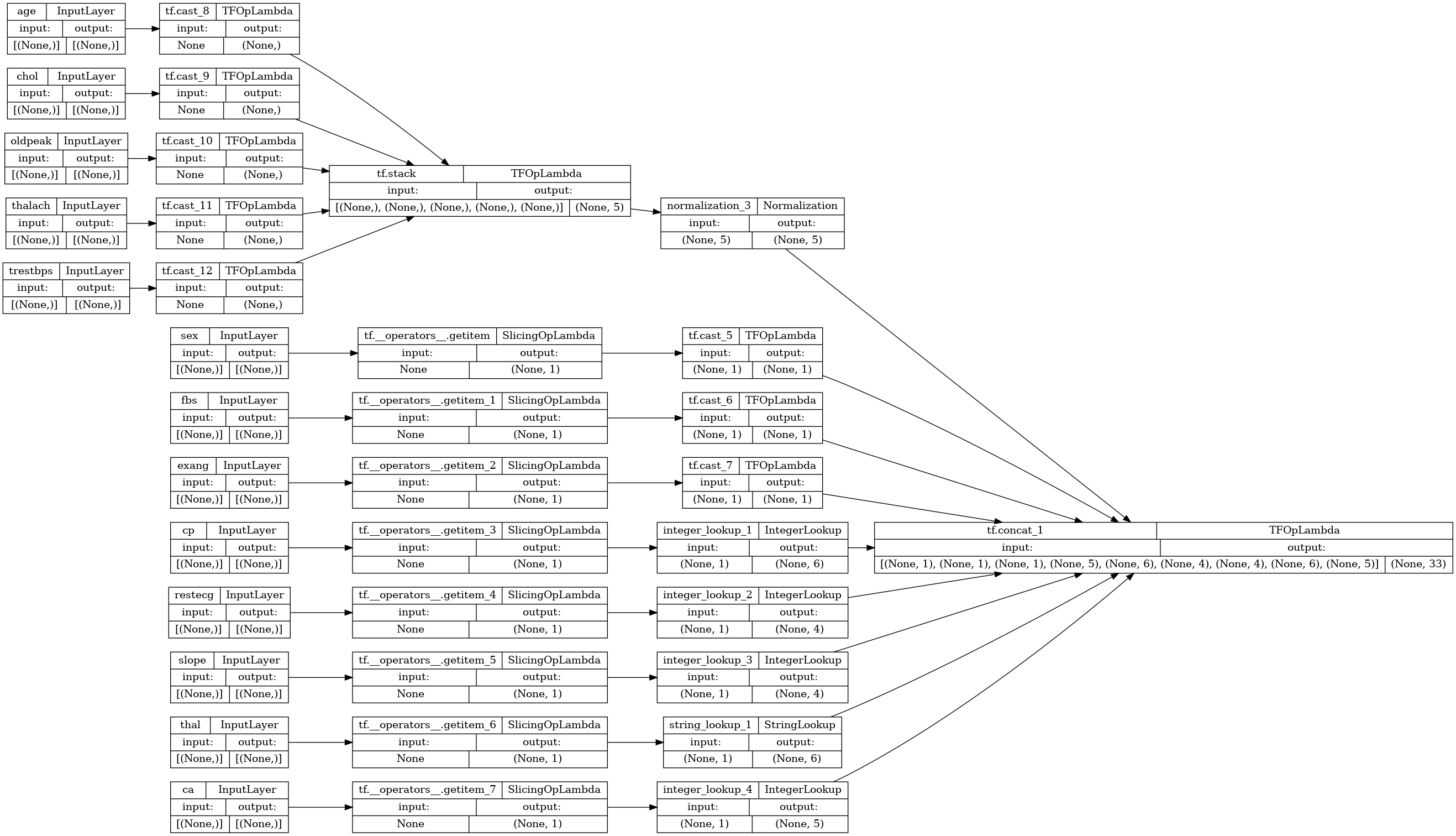
プリプロセッサをテストするには、DataFrame.iloc アクセサを使用して、DataFrame から最初のサンプルをスライスします。次に、それをディクショナリに変換し、ディクショナリをプリプロセッサに渡します。結果は、バイナリ特徴量、正規化された数値特徴量、およびワンホットカテゴリカル特徴量をこの順序で含む単一のベクトルになります。
preprocessor(dict(df.iloc[:1]))
<tf.Tensor: shape=(1, 33), dtype=float32, numpy=
array([[ 1.        ,  1.        ,  0.        ,  0.93383914, -0.26008663,
         1.0680453 ,  0.03480718,  0.74578077,  0.        ,  0.        ,

         1.        ,  0.        ,  0.        ,  0.        ,  0.        ,
         0.        ,  0.        ,  1.        ,  0.        ,  0.        ,
         0.        ,  1.        ,  0.        ,  0.        ,  0.        ,
         1.        ,  0.        ,  0.        ,  0.        ,  1.        ,
         0.        ,  0.        ,  0.        ]], dtype=float32)>
モデルを作成して訓練する
次に、モデルの本体を作成します。前の例と同じ構成を使用します。分類には、いくつかの Dense 正規化線形レイヤーと Dense(1) 出力レイヤーを使用します。
body = tf.keras.Sequential([
  tf.keras.layers.Dense(10, activation='relu'),
  tf.keras.layers.Dense(10, activation='relu'),
  tf.keras.layers.Dense(1)
])
次に、Keras 関数型 API を使用して 2 つの部分を組み合わせます。
inputs
{'age': <KerasTensor: shape=(None,) dtype=float32 (created by layer 'age')>,
 'sex': <KerasTensor: shape=(None,) dtype=int64 (created by layer 'sex')>,
 'cp': <KerasTensor: shape=(None,) dtype=int64 (created by layer 'cp')>,
 'trestbps': <KerasTensor: shape=(None,) dtype=float32 (created by layer 'trestbps')>,
 'chol': <KerasTensor: shape=(None,) dtype=float32 (created by layer 'chol')>,
 'fbs': <KerasTensor: shape=(None,) dtype=int64 (created by layer 'fbs')>,
 'restecg': <KerasTensor: shape=(None,) dtype=int64 (created by layer 'restecg')>,
 'thalach': <KerasTensor: shape=(None,) dtype=float32 (created by layer 'thalach')>,
 'exang': <KerasTensor: shape=(None,) dtype=int64 (created by layer 'exang')>,
 'oldpeak': <KerasTensor: shape=(None,) dtype=float32 (created by layer 'oldpeak')>,
 'slope': <KerasTensor: shape=(None,) dtype=int64 (created by layer 'slope')>,
 'ca': <KerasTensor: shape=(None,) dtype=int64 (created by layer 'ca')>,
 'thal': <KerasTensor: shape=(None,) dtype=string (created by layer 'thal')>}
x = preprocessor(inputs)
x
<KerasTensor: shape=(None, 33) dtype=float32 (created by layer 'model_1')>
result = body(x)
result
<KerasTensor: shape=(None, 1) dtype=float32 (created by layer 'sequential_3')>
model = tf.keras.Model(inputs, result)

model.compile(optimizer='adam',
                loss=tf.keras.losses.BinaryCrossentropy(from_logits=True),
                metrics=['accuracy'])
このモデルは、入力のディクショナリを想定しています。データを渡す最も簡単な方法は、DataFrame を dict に変換し、その dict を x 引数として Model.fit に渡すことです。
history = model.fit(dict(df), target, epochs=5, batch_size=BATCH_SIZE)
Epoch 1/5
152/152 [==============================] - 2s 4ms/step - loss: 0.6485 - accuracy: 0.7162
Epoch 2/5
152/152 [==============================] - 1s 4ms/step - loss: 0.5266 - accuracy: 0.7261
Epoch 3/5
152/152 [==============================] - 1s 4ms/step - loss: 0.4411 - accuracy: 0.7426
Epoch 4/5
152/152 [==============================] - 1s 4ms/step - loss: 0.3844 - accuracy: 0.7855
Epoch 5/5
152/152 [==============================] - 1s 4ms/step - loss: 0.3540 - accuracy: 0.8119
tf.data を使用しても同様に機能します。
ds = tf.data.Dataset.from_tensor_slices((
    dict(df),
    target
))

ds = ds.batch(BATCH_SIZE)
import pprint

for x, y in ds.take(1):
  pprint.pprint(x)
  print()
  print(y)
{'age': <tf.Tensor: shape=(2,), dtype=int64, numpy=array([63, 67])>,
 'ca': <tf.Tensor: shape=(2,), dtype=int64, numpy=array([0, 3])>,
 'chol': <tf.Tensor: shape=(2,), dtype=int64, numpy=array([233, 286])>,
 'cp': <tf.Tensor: shape=(2,), dtype=int64, numpy=array([1, 4])>,
 'exang': <tf.Tensor: shape=(2,), dtype=int64, numpy=array([0, 1])>,
 'fbs': <tf.Tensor: shape=(2,), dtype=int64, numpy=array([1, 0])>,
 'oldpeak': <tf.Tensor: shape=(2,), dtype=float64, numpy=array([2.3, 1.5])>,
 'restecg': <tf.Tensor: shape=(2,), dtype=int64, numpy=array([2, 2])>,
 'sex': <tf.Tensor: shape=(2,), dtype=int64, numpy=array([1, 1])>,
 'slope': <tf.Tensor: shape=(2,), dtype=int64, numpy=array([3, 2])>,
 'thal': <tf.Tensor: shape=(2,), dtype=string, numpy=array([b'fixed', b'normal'], dtype=object)>,
 'thalach': <tf.Tensor: shape=(2,), dtype=int64, numpy=array([150, 108])>,
 'trestbps': <tf.Tensor: shape=(2,), dtype=int64, numpy=array([145, 160])>}

tf.Tensor([0 1], shape=(2,), dtype=int64)
history = model.fit(ds, epochs=5)
Epoch 1/5
152/152 [==============================] - 1s 4ms/step - loss: 0.3320 - accuracy: 0.8317
Epoch 2/5
152/152 [==============================] - 1s 4ms/step - loss: 0.3177 - accuracy: 0.8449
Epoch 3/5
152/152 [==============================] - 1s 4ms/step - loss: 0.3067 - accuracy: 0.8581
Epoch 4/5
152/152 [==============================] - 1s 5ms/step - loss: 0.2979 - accuracy: 0.8581
Epoch 5/5
152/152 [==============================] - 1s 4ms/step - loss: 0.2905 - accuracy: 0.8581