
| | |  GitHub에서 보기 GitHub에서 보기 | |
0 값이 많이 포함된 텐서로 작업할 때 공간 및 시간 효율적인 방식으로 저장하는 것이 중요합니다. 희소 텐서는 0 값이 많이 포함된 텐서를 효율적으로 저장하고 처리할 수 있도록 합니다. 스파스 텐서는 NLP 애플리케이션에서 데이터 사전 처리의 일부로 TF-IDF 와 같은 인코딩 방식과 컴퓨터 비전 애플리케이션에서 어두운 픽셀이 많은 이미지를 사전 처리하는 데 광범위하게 사용됩니다.
TensorFlow의 희소 텐서
TensorFlow는 tf.SparseTensor 객체를 통해 희소 텐서를 나타냅니다. 현재 TensorFlow의 희소 텐서는 좌표 목록(COO) 형식을 사용하여 인코딩됩니다. 이 인코딩 형식은 임베딩과 같은 초희소 행렬에 최적화되어 있습니다.
희소 텐서에 대한 COO 인코딩은 다음으로 구성됩니다.
-
values: 0이 아닌 모든 값을 포함하는[N]모양의 1D 텐서. -
indices: 0이 아닌 값의 인덱스를 포함하는[N, rank]모양의 2D 텐서. -
dense_shape: 텐서의 모양을 지정하는[rank]모양의 1D 텐서.
tf.SparseTensor 컨텍스트에서 0이 아닌 값은 명시적으로 인코딩되지 않은 값입니다. COO 희소 행렬의 values 에 0 값을 명시적으로 포함하는 것이 가능하지만 이러한 "명시적 0"은 일반적으로 희소 텐서에서 0이 아닌 값을 참조할 때 포함되지 않습니다.
tf.SparseTensor 만들기
values , indices 및 dense_shape 를 직접 지정하여 희소 텐서를 구성합니다.
import tensorflow as tf
st1 = tf.SparseTensor(indices=[[0, 3], [2, 4]],
                      values=[10, 20],
                      dense_shape=[3, 10])
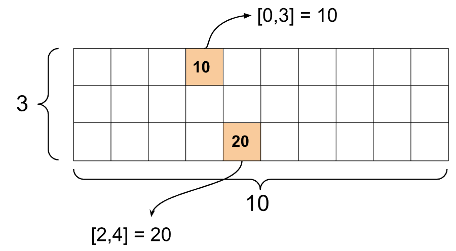
희소 텐서를 인쇄하기 위해 print() 함수를 사용하면 세 가지 구성 요소 텐서의 내용이 표시됩니다.
print(st1)
SparseTensor(indices=tf.Tensor(
[[0 3]
 [2 4]], shape=(2, 2), dtype=int64), values=tf.Tensor([10 20], shape=(2,), dtype=int32), dense_shape=tf.Tensor([ 3 10], shape=(2,), dtype=int64))
0이 아닌 values 이 해당 indices 와 정렬되어 있으면 희소 텐서의 내용을 더 쉽게 이해할 수 있습니다. 0이 아닌 각 값이 자체 줄에 표시되도록 희소 텐서를 예쁘게 인쇄하는 도우미 함수를 정의합니다.
def pprint_sparse_tensor(st):
  s = "<SparseTensor shape=%s \n values={" % (st.dense_shape.numpy().tolist(),)
  for (index, value) in zip(st.indices, st.values):
    s += f"\n  %s: %s" % (index.numpy().tolist(), value.numpy().tolist())
  return s + "}>"
print(pprint_sparse_tensor(st1))
<SparseTensor shape=[3, 10]
 values={
  [0, 3]: 10
  [2, 4]: 20}>
tf.sparse.from_dense 를 사용하여 조밀 텐서에서 희소 텐서를 구성하고 tf.sparse.from_dense 를 사용하여 조밀 텐서로 다시 변환할 tf.sparse.to_dense 있습니다.
st2 = tf.sparse.from_dense([[1, 0, 0, 8], [0, 0, 0, 0], [0, 0, 3, 0]])
print(pprint_sparse_tensor(st2))
<SparseTensor shape=[3, 4]
 values={
  [0, 0]: 1
  [0, 3]: 8
  [2, 2]: 3}>
st3 = tf.sparse.to_dense(st2)
print(st3)
tf.Tensor(
[[1 0 0 8]
 [0 0 0 0]
 [0 0 3 0]], shape=(3, 4), dtype=int32)
희소 텐서 조작
tf.sparse 패키지의 유틸리티를 사용하여 희소 텐서를 조작하십시오. 조밀한 텐서의 산술 조작에 사용할 수 있는 tf.math.add 와 같은 연산은 희소 텐서에서 작동하지 않습니다.
tf.sparse.add 를 사용하여 동일한 모양의 희소 텐서를 추가합니다.
st_a = tf.SparseTensor(indices=[[0, 2], [3, 4]],
                       values=[31, 2],
                       dense_shape=[4, 10])

st_b = tf.SparseTensor(indices=[[0, 2], [7, 0]],
                       values=[56, 38],
                       dense_shape=[4, 10])

st_sum = tf.sparse.add(st_a, st_b)

print(pprint_sparse_tensor(st_sum))
<SparseTensor shape=[4, 10]
 values={
  [0, 2]: 87
  [3, 4]: 2
  [7, 0]: 38}>
tf.sparse.sparse_dense_matmul 을 사용하여 희소 텐서를 고밀도 행렬과 곱합니다.
st_c = tf.SparseTensor(indices=([0, 1], [1, 0], [1, 1]),
                       values=[13, 15, 17],
                       dense_shape=(2,2))

mb = tf.constant([[4], [6]])
product = tf.sparse.sparse_dense_matmul(st_c, mb)

print(product)
tf.Tensor(
[[ 78]
 [162]], shape=(2, 1), dtype=int32)
tf.sparse.concat 을 사용하여 희소 텐서를 함께 tf.sparse.concat 를 사용하여 tf.sparse.slice 합니다.
sparse_pattern_A = tf.SparseTensor(indices = [[2,4], [3,3], [3,4], [4,3], [4,4], [5,4]],
                         values = [1,1,1,1,1,1],
                         dense_shape = [8,5])
sparse_pattern_B = tf.SparseTensor(indices = [[0,2], [1,1], [1,3], [2,0], [2,4], [2,5], [3,5],
                                              [4,5], [5,0], [5,4], [5,5], [6,1], [6,3], [7,2]],
                         values = [1,1,1,1,1,1,1,1,1,1,1,1,1,1],
                         dense_shape = [8,6])
sparse_pattern_C = tf.SparseTensor(indices = [[3,0], [4,0]],
                         values = [1,1],
                         dense_shape = [8,6])

sparse_patterns_list = [sparse_pattern_A, sparse_pattern_B, sparse_pattern_C]
sparse_pattern = tf.sparse.concat(axis=1, sp_inputs=sparse_patterns_list)
print(tf.sparse.to_dense(sparse_pattern))
tf.Tensor(
[[0 0 0 0 0 0 0 1 0 0 0 0 0 0 0 0 0]
 [0 0 0 0 0 0 1 0 1 0 0 0 0 0 0 0 0]
 [0 0 0 0 1 1 0 0 0 1 1 0 0 0 0 0 0]
 [0 0 0 1 1 0 0 0 0 0 1 1 0 0 0 0 0]
 [0 0 0 1 1 0 0 0 0 0 1 1 0 0 0 0 0]
 [0 0 0 0 1 1 0 0 0 1 1 0 0 0 0 0 0]
 [0 0 0 0 0 0 1 0 1 0 0 0 0 0 0 0 0]
 [0 0 0 0 0 0 0 1 0 0 0 0 0 0 0 0 0]], shape=(8, 17), dtype=int32)
sparse_slice_A = tf.sparse.slice(sparse_pattern_A, start = [0,0], size = [8,5])
sparse_slice_B = tf.sparse.slice(sparse_pattern_B, start = [0,5], size = [8,6])
sparse_slice_C = tf.sparse.slice(sparse_pattern_C, start = [0,10], size = [8,6])
print(tf.sparse.to_dense(sparse_slice_A))
print(tf.sparse.to_dense(sparse_slice_B))
print(tf.sparse.to_dense(sparse_slice_C))
tf.Tensor(
[[0 0 0 0 0]
 [0 0 0 0 0]
 [0 0 0 0 1]
 [0 0 0 1 1]
 [0 0 0 1 1]
 [0 0 0 0 1]
 [0 0 0 0 0]
 [0 0 0 0 0]], shape=(8, 5), dtype=int32)
tf.Tensor(
[[0]
 [0]
 [1]
 [1]
 [1]
 [1]
 [0]
 [0]], shape=(8, 1), dtype=int32)
tf.Tensor([], shape=(8, 0), dtype=int32)
TensorFlow 2.4 이상을 사용하는 경우 희소 텐서의 0이 아닌 값에 대한 요소별 연산에 tf.sparse.map_values 를 사용하세요.
st2_plus_5 = tf.sparse.map_values(tf.add, st2, 5)
print(tf.sparse.to_dense(st2_plus_5))
tf.Tensor(
[[ 6  0  0 13]
 [ 0  0  0  0]
 [ 0  0  8  0]], shape=(3, 4), dtype=int32)
0이 아닌 값만 수정되었다는 점에 유의하십시오. 0 값은 0으로 유지됩니다.
마찬가지로 이전 버전의 TensorFlow에 대해 아래 디자인 패턴을 따를 수 있습니다.
st2_plus_5 = tf.SparseTensor(
    st2.indices,
    st2.values + 5,
    st2.dense_shape)
print(tf.sparse.to_dense(st2_plus_5))
tf.Tensor(
[[ 6  0  0 13]
 [ 0  0  0  0]
 [ 0  0  8  0]], shape=(3, 4), dtype=int32)
다른 TensorFlow API와 함께 tf.SparseTensor 사용
희소 텐서는 다음 TensorFlow API와 투명하게 작동합니다.
-
tf.keras -
tf.data -
tf.Train.Exampleprotobuf -
tf.function -
tf.while_loop -
tf.cond -
tf.identity -
tf.cast -
tf.print -
tf.saved_model -
tf.io.serialize_sparse -
tf.io.serialize_many_sparse -
tf.io.deserialize_many_sparse -
tf.math.abs -
tf.math.negative -
tf.math.sign -
tf.math.square -
tf.math.sqrt -
tf.math.erf -
tf.math.tanh -
tf.math.bessel_i0e -
tf.math.bessel_i1e
위의 API 중 일부에 대한 예가 아래에 나와 있습니다.
tf.keras
tf.keras API의 하위 집합은 값비싼 캐스팅 또는 변환 작업 없이 희소 텐서를 지원합니다. Keras API를 사용하면 희소 텐서를 Keras 모델에 대한 입력으로 전달할 수 있습니다. tf.keras.Input 또는 tf.keras.layers.InputLayer 를 호출할 때 sparse=True 로 설정합니다. Keras 계층 간에 희소 텐서를 전달할 수 있으며 Keras 모델이 이를 출력으로 반환하도록 할 수도 있습니다. 모델의 tf.keras.layers.Dense 레이어에서 희소 텐서를 사용하면 밀도가 높은 텐서를 출력합니다.
아래 예는 희소 입력을 지원하는 계층만 사용하는 경우 희소 텐서를 Keras 모델에 대한 입력으로 전달하는 방법을 보여줍니다.
x = tf.keras.Input(shape=(4,), sparse=True)
y = tf.keras.layers.Dense(4)(x)
model = tf.keras.Model(x, y)

sparse_data = tf.SparseTensor(
    indices = [(0,0),(0,1),(0,2),
               (4,3),(5,0),(5,1)],
    values = [1,1,1,1,1,1],
    dense_shape = (6,4)
)

model(sparse_data)

model.predict(sparse_data)
array([[-1.3111044 , -1.7598825 ,  0.07225233, -0.44544357],
       [ 0.        ,  0.        ,  0.        ,  0.        ],
       [ 0.        ,  0.        ,  0.        ,  0.        ],
       [ 0.        ,  0.        ,  0.        ,  0.        ],
       [ 0.8517609 , -0.16835624,  0.7307872 , -0.14531797],
       [-0.8916302 , -0.9417639 ,  0.24563438, -0.9029659 ]],
      dtype=float32)
tf.data
tf.data API를 사용하면 간단하고 재사용 가능한 부분에서 복잡한 입력 파이프라인을 구축할 수 있습니다. 핵심 데이터 구조는 각 요소가 하나 이상의 구성 요소로 구성된 요소 시퀀스를 나타내는 tf.data.Dataset 입니다.
희소 텐서를 사용하여 데이터세트 빌드
tf.data.Dataset.from_tensor_slices tf.Tensor NumPy 배열에서 구축하는 데 사용되는 것과 동일한 방법을 사용하여 희소 텐서에서 데이터세트를 구축합니다. 이 연산은 데이터의 희소성(또는 희소성)을 보존합니다.
dataset = tf.data.Dataset.from_tensor_slices(sparse_data)
for element in dataset:
  print(pprint_sparse_tensor(element))
<SparseTensor shape=[4]
 values={
  [0]: 1
  [1]: 1
  [2]: 1}>
<SparseTensor shape=[4]
 values={}>
<SparseTensor shape=[4]
 values={}>
<SparseTensor shape=[4]
 values={}>
<SparseTensor shape=[4]
 values={
  [3]: 1}>
<SparseTensor shape=[4]
 values={
  [0]: 1
  [1]: 1}>
희소 텐서를 사용한 데이터 세트 일괄 처리 및 일괄 해제
Dataset.batch 및 Dataset.unbatch 메서드를 각각 사용하여 희소 텐서를 사용하여 데이터 세트를 일괄 처리(연속 요소를 단일 요소로 결합)하고 일괄 처리 해제할 수 있습니다.
batched_dataset = dataset.batch(2)
for element in batched_dataset:
  print (pprint_sparse_tensor(element))
<SparseTensor shape=[2, 4]
 values={
  [0, 0]: 1
  [0, 1]: 1
  [0, 2]: 1}>
<SparseTensor shape=[2, 4]
 values={}>
<SparseTensor shape=[2, 4]
 values={
  [0, 3]: 1
  [1, 0]: 1
  [1, 1]: 1}>
unbatched_dataset = batched_dataset.unbatch()
for element in unbatched_dataset:
  print (pprint_sparse_tensor(element))
<SparseTensor shape=[4]
 values={
  [0]: 1
  [1]: 1
  [2]: 1}>
<SparseTensor shape=[4]
 values={}>
<SparseTensor shape=[4]
 values={}>
<SparseTensor shape=[4]
 values={}>
<SparseTensor shape=[4]
 values={
  [3]: 1}>
<SparseTensor shape=[4]
 values={
  [0]: 1
  [1]: 1}>
tf.data.experimental.dense_to_sparse_batch 를 사용하여 다양한 모양의 데이터 세트 요소를 희소 텐서로 일괄 처리할 수도 있습니다.
희소 텐서를 사용하여 데이터 세트 변환
Dataset.map 을 사용하여 Datasets에서 희소 텐서를 변환하고 생성합니다.
transform_dataset = dataset.map(lambda x: x*2)
for i in transform_dataset:
  print(pprint_sparse_tensor(i))
<SparseTensor shape=[4]
 values={
  [0]: 2
  [1]: 2
  [2]: 2}>
<SparseTensor shape=[4]
 values={}>
<SparseTensor shape=[4]
 values={}>
<SparseTensor shape=[4]
 values={}>
<SparseTensor shape=[4]
 values={
  [3]: 2}>
<SparseTensor shape=[4]
 values={
  [0]: 2
  [1]: 2}>
tf.train.Example
tf.train.Example 은 TensorFlow 데이터에 대한 표준 protobuf 인코딩입니다. tf.train.Example 과 함께 희소 텐서를 사용할 때 다음을 수행할 수 있습니다.
tf.io.VarLenFeature 를 사용하여 가변 길이 데이터를
tf.SparseTensor로tf.io.VarLenFeature. 그러나 대신tf.io.RaggedFeature사용을 고려해야 합니다.tf.io.SparseFeature를 사용하여 임의의 희소 데이터를tf.SparseTensor로 읽어들입니다. tf.io.SparseFeature는 3개의 개별 기능 키를 사용하여indices,values및dense_shape를 저장합니다.
tf.function
tf.function 데코레이터는 Python 함수에 대한 TensorFlow 그래프를 미리 계산하여 TensorFlow 코드의 성능을 크게 향상시킬 수 있습니다. 희소 텐서는 tf.function 및 구체 함수 모두에서 투명하게 작동합니다.
@tf.function
def f(x,y):
  return tf.sparse.sparse_dense_matmul(x,y)

a = tf.SparseTensor(indices=[[0, 3], [2, 4]],
                    values=[15, 25],
                    dense_shape=[3, 10])

b = tf.sparse.to_dense(tf.sparse.transpose(a))

c = f(a,b)

print(c)
tf.Tensor(
[[225   0   0]
 [  0   0   0]
 [  0   0 625]], shape=(3, 3), dtype=int32)
결측값과 0값 구별하기
tf.SparseTensor 에 대한 대부분의 연산은 결측값과 명시적 0 값을 동일하게 취급합니다. 이것은 의도적으로 설계된 것입니다. tf.SparseTensor 는 조밀한 텐서처럼 작동해야 합니다.
그러나 0 값과 결측값을 구별하는 것이 유용할 수 있는 몇 가지 경우가 있습니다. 특히, 이것은 훈련 데이터에서 누락/알 수 없는 데이터를 인코딩하는 한 가지 방법을 허용합니다. 예를 들어, 일부 누락된 점수와 함께 점수 텐서(-Inf에서 +Inf까지의 모든 부동 소수점 값을 가질 수 있음)가 있는 사용 사례를 고려하십시오. 명시적 0은 알려진 0 점수이지만 암시적 0 값은 실제로 0이 아니라 누락된 데이터를 나타내는 희소 텐서를 사용하여 이 텐서를 인코딩할 수 있습니다.
tf.sparse.reduce_max 와 같은 일부 연산은 누락된 값을 0인 것처럼 취급하지 않습니다. 예를 들어 아래 코드 블록을 실행할 때 예상되는 출력은 0 입니다. 그러나 이 예외로 인해 출력은 -3 입니다.
print(tf.sparse.reduce_max(tf.sparse.from_dense([-5, 0, -3])))
tf.Tensor(-3, shape=(), dtype=int32)
대조적으로 tf.math.reduce_max 를 조밀한 텐서에 적용하면 예상대로 출력이 0이 됩니다.
print(tf.math.reduce_max([-5, 0, -3]))
tf.Tensor(0, shape=(), dtype=int32)
추가 읽을거리 및 리소스
- 텐서에 대해 알아보려면 텐서 가이드 를 참조하세요.
- 비정형 텐서 가이드 를 읽고 비균일 데이터로 작업할 수 있는 텐서 유형인 비정형 텐서를 사용하는 방법을 알아보세요.
-
tf.Example데이터 디코더 에서 희소 텐서를 사용하는 TensorFlow Model Garden 에서 이 객체 감지 모델을 확인하십시오.