
| | |  Xem nguồn trên GitHub Xem nguồn trên GitHub | |
Thành lập
Đầu tiên hãy cài đặt các gói được sử dụng trong bản demo này.
pip install -q dm-sonnet
Nhập (tf, tfp với thủ thuật adjoint, v.v.)
import numpy as np
import tqdm as tqdm
import sklearn.datasets as skd

# visualization
import matplotlib.pyplot as plt
import seaborn as sns
from scipy.stats import kde

# tf and friends
import tensorflow.compat.v2 as tf
import tensorflow_probability as tfp
import sonnet as snt
tf.enable_v2_behavior()

tfb = tfp.bijectors
tfd = tfp.distributions

def make_grid(xmin, xmax, ymin, ymax, gridlines, pts):
  xpts = np.linspace(xmin, xmax, pts)
  ypts = np.linspace(ymin, ymax, pts)
  xgrid = np.linspace(xmin, xmax, gridlines)
  ygrid = np.linspace(ymin, ymax, gridlines)
  xlines = np.stack([a.ravel() for a in np.meshgrid(xpts, ygrid)])
  ylines = np.stack([a.ravel() for a in np.meshgrid(xgrid, ypts)])
  return np.concatenate([xlines, ylines], 1).T

grid = make_grid(-3, 3, -3, 3, 4, 100)
/usr/local/lib/python3.6/dist-packages/statsmodels/tools/_testing.py:19: FutureWarning: pandas.util.testing is deprecated. Use the functions in the public API at pandas.testing instead.
  import pandas.util.testing as tm
Chức năng trợ giúp để trực quan hóa
def plot_density(data, axis):
  x, y = np.squeeze(np.split(data, 2, axis=1))
  levels = np.linspace(0.0, 0.75, 10)
  kwargs = {'levels': levels}
  return sns.kdeplot(x, y, cmap="viridis", shade=True,
                     shade_lowest=True, ax=axis, **kwargs)


def plot_points(data, axis, s=10, color='b', label=''):
  x, y = np.squeeze(np.split(data, 2, axis=1))
  axis.scatter(x, y, c=color, s=s, label=label)


def plot_panel(
    grid, samples, transformed_grid, transformed_samples,
    dataset, axarray, limits=True):
  if len(axarray) != 4:
    raise ValueError('Expected 4 axes for the panel')
  ax1, ax2, ax3, ax4 = axarray
  plot_points(data=grid, axis=ax1, s=20, color='black', label='grid')
  plot_points(samples, ax1, s=30, color='blue', label='samples')
  plot_points(transformed_grid, ax2, s=20, color='black', label='ode(grid)')
  plot_points(transformed_samples, ax2, s=30, color='blue', label='ode(samples)')
  ax3 = plot_density(transformed_samples, ax3)
  ax4 = plot_density(dataset, ax4)
  if limits:
    set_limits([ax1], -3.0, 3.0, -3.0, 3.0)
    set_limits([ax2], -2.0, 3.0, -2.0, 3.0)
    set_limits([ax3, ax4], -1.5, 2.5, -0.75, 1.25)


def set_limits(axes, min_x, max_x, min_y, max_y):
  if isinstance(axes, list):
    for axis in axes:
      set_limits(axis, min_x, max_x, min_y, max_y)
  else:
    axes.set_xlim(min_x, max_x)
    axes.set_ylim(min_y, max_y)
FFJORD bijector
Trong chuyên mục này, chúng tôi trình diễn bijector FFJORD, được đề xuất ban đầu trong bài báo của Grathwohl, Will, et al. arXiv liên kết .
Trong Tóm lại ý tưởng đằng sau cách tiếp cận như vậy là để thiết lập một sự tương ứng giữa một bản phân phối cơ sở biết và phân phối dữ liệu.
Để thiết lập kết nối này, chúng ta cần
- Xác định một song ánh bản đồ \(\mathcal{T}_{\theta}:\mathbf{x} \rightarrow \mathbf{y}\), \(\mathcal{T}_{\theta}^{1}:\mathbf{y} \rightarrow \mathbf{x}\) giữa không gian \(\mathcal{Y}\) trên đó phân phối cơ sở được xác định và không gian \(\mathcal{X}\) của miền dữ liệu.
- Hiệu quả theo dõi các biến dạng chúng tôi thực hiện để chuyển khái niệm xác suất vào \(\mathcal{X}\).
Điều kiện thứ hai được chính thức hóa trong biểu thức sau đây để phân bố xác suất xác định trên \(\mathcal{X}\):
\[ \log p_{\mathbf{x} }(\mathbf{x})=\log p_{\mathbf{y} }(\mathbf{y})-\log \operatorname{det}\left|\frac{\partial \mathcal{T}_{\theta}(\mathbf{y})}{\partial \mathbf{y} }\right| \]
FFJORD bijector thực hiện điều này bằng cách xác định một phép biến đổi
\[ \mathcal{T_{\theta} }: \mathbf{x} = \mathbf{z}(t_{0}) \rightarrow \mathbf{y} = \mathbf{z}(t_{1}) \quad : \quad \frac{d \mathbf{z} }{dt} = \mathbf{f}(t, \mathbf{z}, \theta) \]
Chuyển đổi này là khả nghịch, miễn là chức năng \(\mathbf{f}\) mô tả sự phát triển của nhà nước \(\mathbf{z}\) được cư xử tốt và log_det_jacobian thể được tính toán bằng cách tích hợp các biểu thức sau đây.
\[ \log \operatorname{det}\left|\frac{\partial \mathcal{T}_{\theta}(\mathbf{y})}{\partial \mathbf{y} }\right| = -\int_{t_{0} }^{t_{1} } \operatorname{Tr}\left(\frac{\partial \mathbf{f}(t, \mathbf{z}, \theta)}{\partial \mathbf{z}(t)}\right) d t \]
Trong bản demo này, chúng tôi sẽ đào tạo một bijector FFJORD để warp một phân bố gaussian vào sự phân bố xác định bởi moons tập dữ liệu. Điều này sẽ được thực hiện trong 3 bước:
- Xác định phân phối cơ sở
- Xác định bijector FFJORD
- Giảm thiểu khả năng ghi nhật ký chính xác của tập dữ liệu
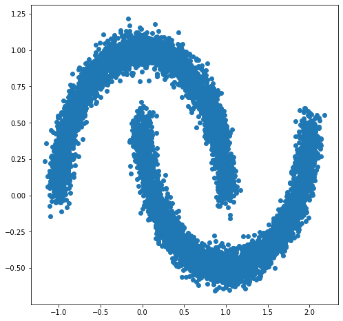
Đầu tiên, chúng tôi tải dữ liệu
Dataset
DATASET_SIZE = 1024 * 8
BATCH_SIZE = 256
SAMPLE_SIZE = DATASET_SIZE

moons = skd.make_moons(n_samples=DATASET_SIZE, noise=.06)[0]

moons_ds = tf.data.Dataset.from_tensor_slices(moons.astype(np.float32))
moons_ds = moons_ds.prefetch(tf.data.experimental.AUTOTUNE)
moons_ds = moons_ds.cache()
moons_ds = moons_ds.shuffle(DATASET_SIZE)
moons_ds = moons_ds.batch(BATCH_SIZE)

plt.figure(figsize=[8, 8])
plt.scatter(moons[:, 0], moons[:, 1])
plt.show()
Tiếp theo, chúng tôi khởi tạo một phân phối cơ sở
base_loc = np.array([0.0, 0.0]).astype(np.float32)
base_sigma = np.array([0.8, 0.8]).astype(np.float32)
base_distribution = tfd.MultivariateNormalDiag(base_loc, base_sigma)
Chúng tôi sử dụng nhiều lớp Perceptron để mô hình state_derivative_fn .
Trong khi không cần thiết cho tập dữ liệu này, nó thường benefitial để làm state_derivative_fn phụ thuộc vào thời gian. Ở đây chúng ta đạt được điều này bằng cách kết hợp t việc xâm nhập của mạng của chúng tôi.
class MLP_ODE(snt.Module):
  """Multi-layer NN ode_fn."""
  def __init__(self, num_hidden, num_layers, num_output, name='mlp_ode'):
    super(MLP_ODE, self).__init__(name=name)
    self._num_hidden = num_hidden
    self._num_output = num_output
    self._num_layers = num_layers
    self._modules = []
    for _ in range(self._num_layers - 1):
      self._modules.append(snt.Linear(self._num_hidden))
      self._modules.append(tf.math.tanh)
    self._modules.append(snt.Linear(self._num_output))
    self._model = snt.Sequential(self._modules)

  def __call__(self, t, inputs):
    inputs = tf.concat([tf.broadcast_to(t, inputs.shape), inputs], -1)
    return self._model(inputs)
Các thông số mô hình và đào tạo
LR = 1e-2
NUM_EPOCHS = 80
STACKED_FFJORDS = 4
NUM_HIDDEN = 8
NUM_LAYERS = 3
NUM_OUTPUT = 2
Bây giờ chúng ta xây dựng một chồng các bijector FFJORD. Mỗi bijector được cung cấp với ode_solve_fn và trace_augmentation_fn và nó riêng state_derivative_fn mô hình, vì vậy mà họ đại diện cho một chuỗi các biến đổi khác nhau.
Xây dựng bijector
solver = tfp.math.ode.DormandPrince(atol=1e-5)
ode_solve_fn = solver.solve
trace_augmentation_fn = tfb.ffjord.trace_jacobian_exact

bijectors = []
for _ in range(STACKED_FFJORDS):
  mlp_model = MLP_ODE(NUM_HIDDEN, NUM_LAYERS, NUM_OUTPUT)
  next_ffjord = tfb.FFJORD(
      state_time_derivative_fn=mlp_model,ode_solve_fn=ode_solve_fn,
      trace_augmentation_fn=trace_augmentation_fn)
  bijectors.append(next_ffjord)

stacked_ffjord = tfb.Chain(bijectors[::-1])
Bây giờ chúng ta có thể sử dụng TransformedDistribution mà là kết quả của cong vênh base_distribution với stacked_ffjord bijector.
transformed_distribution = tfd.TransformedDistribution(
    distribution=base_distribution, bijector=stacked_ffjord)
Bây giờ chúng tôi xác định quy trình đào tạo của chúng tôi. Chúng tôi chỉ đơn giản là giảm thiểu khả năng ghi nhật ký tiêu cực của dữ liệu.
Tập huấn
@tf.function
def train_step(optimizer, target_sample):
  with tf.GradientTape() as tape:
    loss = -tf.reduce_mean(transformed_distribution.log_prob(target_sample))
  variables = tape.watched_variables()
  gradients = tape.gradient(loss, variables)
  optimizer.apply(gradients, variables)
  return loss
Mẫu
@tf.function
def get_samples():
  base_distribution_samples = base_distribution.sample(SAMPLE_SIZE)
  transformed_samples = transformed_distribution.sample(SAMPLE_SIZE)
  return base_distribution_samples, transformed_samples


@tf.function
def get_transformed_grid():
  transformed_grid = stacked_ffjord.forward(grid)
  return transformed_grid
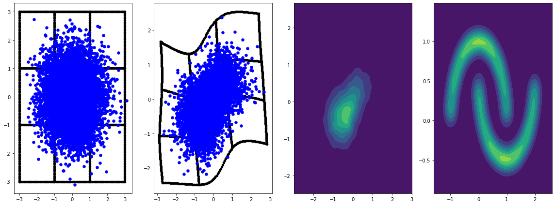
Lập đồ thị các mẫu từ các phân bố cơ sở và được biến đổi.
evaluation_samples = []
base_samples, transformed_samples = get_samples()
transformed_grid = get_transformed_grid()
evaluation_samples.append((base_samples, transformed_samples, transformed_grid))
WARNING:tensorflow:From /usr/local/lib/python3.6/dist-packages/tensorflow/python/ops/resource_variable_ops.py:1817: calling BaseResourceVariable.__init__ (from tensorflow.python.ops.resource_variable_ops) with constraint is deprecated and will be removed in a future version.
Instructions for updating:
If using Keras pass *_constraint arguments to layers.
panel_id = 0
panel_data = evaluation_samples[panel_id]
fig, axarray = plt.subplots(
  1, 4, figsize=(16, 6))
plot_panel(
    grid, panel_data[0], panel_data[2], panel_data[1], moons, axarray, False)
plt.tight_layout()
learning_rate = tf.Variable(LR, trainable=False)
optimizer = snt.optimizers.Adam(learning_rate)

for epoch in tqdm.trange(NUM_EPOCHS // 2):
  base_samples, transformed_samples = get_samples()
  transformed_grid = get_transformed_grid()
  evaluation_samples.append(
      (base_samples, transformed_samples, transformed_grid))
  for batch in moons_ds:
    _ = train_step(optimizer, batch)
0%|          | 0/40 [00:00<?, ?it/s]
WARNING:tensorflow:From /usr/local/lib/python3.6/dist-packages/tensorflow_probability/python/math/ode/base.py:350: calling while_loop_v2 (from tensorflow.python.ops.control_flow_ops) with back_prop=False is deprecated and will be removed in a future version.
Instructions for updating:
back_prop=False is deprecated. Consider using tf.stop_gradient instead.
Instead of:
results = tf.while_loop(c, b, vars, back_prop=False)
Use:
results = tf.nest.map_structure(tf.stop_gradient, tf.while_loop(c, b, vars))
100%|██████████| 40/40 [07:00<00:00, 10.52s/it]
panel_id = -1
panel_data = evaluation_samples[panel_id]
fig, axarray = plt.subplots(
  1, 4, figsize=(16, 6))
plot_panel(grid, panel_data[0], panel_data[2], panel_data[1], moons, axarray)
plt.tight_layout()
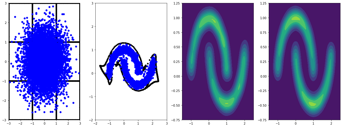
Đào tạo nó lâu hơn với tỷ lệ học tập dẫn đến cải thiện hơn nữa.
Không được đề cập trong ví dụ này, FFJORD bijector hỗ trợ ước tính dấu vết ngẫu nhiên của hutchinson. Người lập dự toán cụ thể có thể được cung cấp qua trace_augmentation_fn . Tương tự như vậy các nhà tích hợp thay thế có thể được sử dụng bằng cách định nghĩa tùy chỉnh ode_solve_fn .