
| | |  GitHub पर स्रोत देखें GitHub पर स्रोत देखें | |
इस कोलाब में, हम TensorFlow और TensorFlow प्रायिकता का उपयोग करके गाऊसी प्रक्रिया प्रतिगमन का पता लगाते हैं। हम कुछ ज्ञात कार्यों से कुछ शोर अवलोकन उत्पन्न करते हैं और उन डेटा में जीपी मॉडल फिट करते हैं। हम तब जीपी पोस्टीरियर से नमूना लेते हैं और उनके डोमेन में ग्रिड पर नमूना फ़ंक्शन मानों को प्लॉट करते हैं।
पृष्ठभूमि
चलो \(\mathcal{X}\) किसी भी सेट हो। एक गाऊसी प्रक्रिया (जीपी) द्वारा अनुक्रमित यादृच्छिक परिवर्तनीय का एक संग्रह है \(\mathcal{X}\) ऐसी है कि अगर\(\{X_1, \ldots, X_n\} \subset \mathcal{X}\) किसी भी परिमित सबसेट है, सीमांत घनत्व\(p(X_1 = x_1, \ldots, X_n = x_n)\) मल्टीवेरिएट है गाऊसी। किसी भी गाऊसी वितरण को उसके पहले और दूसरे केंद्रीय क्षणों (माध्य और सहप्रसरण) द्वारा पूरी तरह से निर्दिष्ट किया जाता है, और जीपी कोई अपवाद नहीं है। हम अपने मतलब समारोह के मामले में पूरी तरह से एक जीपी निर्दिष्ट कर सकते हैं \(\mu : \mathcal{X} \to \mathbb{R}\) और सहप्रसरण समारोह\(k : \mathcal{X} \times \mathcal{X} \to \mathbb{R}\)। GP की अधिकांश अभिव्यंजक शक्ति सहप्रसरण फलन के चुनाव में समाहित है। विभिन्न कारणों से, सहप्रसरण समारोह भी एक कर्नेल समारोह के रूप में जाना जाता है। यह केवल सममित और सकारात्मक-निश्चित होना करने के लिए (देखें आवश्यक है अ। रासमुसेन और विलियम्स के 4 )। नीचे हम घातांक द्विघात सहप्रसरण कर्नेल का उपयोग करते हैं। इसका रूप है
\[ k(x, x') := \sigma^2 \exp \left( \frac{\|x - x'\|^2}{\lambda^2} \right) \]
जहां \(\sigma^2\) 'आयाम' और कहा जाता है \(\lambda\) लंबाई पैमाने। कर्नेल मापदंडों को अधिकतम संभावना अनुकूलन प्रक्रिया के माध्यम से चुना जा सकता है।
एक जीपी से एक पूर्ण नमूना पूरी जगह पर एक वास्तविक मूल्य समारोह शामिल\(\mathcal{X}\) और अभ्यास का एहसास करने अव्यावहारिक में है; अक्सर कोई उन बिंदुओं का एक सेट चुनता है जिस पर नमूना देखने के लिए और इन बिंदुओं पर फ़ंक्शन मान खींचता है। यह एक उपयुक्त (परिमित-आयामी) बहु-भिन्न गाऊसी से नमूना लेकर प्राप्त किया जाता है।
ध्यान दें कि, उपरोक्त परिभाषा के अनुसार, कोई भी परिमित-आयामी बहुभिन्नरूपी गाऊसी वितरण भी एक गाऊसी प्रक्रिया है। आमतौर पर, जब एक एक जीपी को संदर्भित करता है, यह निहित है कि सूचकांक सेट कुछ है \(\mathbb{R}^n\)और हम वास्तव में यहाँ इस धारणा कर देगा।
मशीन सीखने में गाऊसी प्रक्रियाओं का एक सामान्य अनुप्रयोग गाऊसी प्रक्रिया प्रतिगमन है। विचार यह है कि हम एक अज्ञात समारोह को देखते हुए शोर टिप्पणियों अनुमान लगाने के लिए इच्छा \(\{y_1, \ldots, y_N\}\) अंक की एक निश्चित संख्या में समारोह के \(\{x_1, \ldots x_N\}.\) हम एक उत्पादक प्रक्रिया की कल्पना
\[ \begin{align} f \sim \: & \textsf{GaussianProcess}\left( \text{mean_fn}=\mu(x), \text{covariance_fn}=k(x, x')\right) \\ y_i \sim \: & \textsf{Normal}\left( \text{loc}=f(x_i), \text{scale}=\sigma\right), i = 1, \ldots, N \end{align} \]
जैसा कि ऊपर उल्लेख किया गया है, नमूना फ़ंक्शन की गणना करना असंभव है, क्योंकि हमें इसके मूल्य की अनंत संख्या में आवश्यकता होगी। इसके बजाय, एक बहुभिन्नरूपी गाऊसी से एक परिमित नमूने पर विचार करता है।
\[ \begin{gather} \begin{bmatrix} f(x_1) \\ \vdots \\ f(x_N) \end{bmatrix} \sim \textsf{MultivariateNormal} \left( \: \text{loc}= \begin{bmatrix} \mu(x_1) \\ \vdots \\ \mu(x_N) \end{bmatrix} \:,\: \text{scale}= \begin{bmatrix} k(x_1, x_1) & \cdots & k(x_1, x_N) \\ \vdots & \ddots & \vdots \\ k(x_N, x_1) & \cdots & k(x_N, x_N) \\ \end{bmatrix}^{1/2} \: \right) \end{gather} \\ y_i \sim \textsf{Normal} \left( \text{loc}=f(x_i), \text{scale}=\sigma \right) \]
नोट प्रतिपादक \(\frac{1}{2}\) सहप्रसरण मैट्रिक्स पर: यह एक Cholesky अपघटन को दर्शाता है। चोल्स्की की गणना आवश्यक है क्योंकि एमवीएन एक स्थान-पैमाने पर परिवार वितरण है। दुर्भाग्य से Cholesky अपघटन computationally महंगा है, लेने \(O(N^3)\) समय और \(O(N^2)\) अंतरिक्ष। अधिकांश जीपी साहित्य इस प्रतीत होता है कि सहज रूप से छोटे प्रतिपादक से निपटने पर केंद्रित है।
पूर्व माध्य फलन को स्थिर, प्राय: शून्य मान लेना आम बात है। साथ ही, कुछ नोटेशनल कन्वेंशन सुविधाजनक होते हैं। एक अक्सर लिखते हैं \(\mathbf{f}\) नमूना समारोह मूल्यों के परिमित वेक्टर के लिए। दिलचस्प अंकन की एक संख्या सहप्रसरण मैट्रिक्स के आवेदन से उत्पन्न लिए उपयोग किया जाता \(k\) आदानों के जोड़े के लिए। बाद (Quiñonero-Candela, 2005) , हम ध्यान दें कि मैट्रिक्स के घटकों विशेष इनपुट बिंदुओं पर समारोह मूल्यों की सहप्रसरण हैं। इस प्रकार हम सहप्रसरण मैट्रिक्स निरूपित कर सकते हैं के रूप में \(K_{AB}\)जहां \(A\) और \(B\) दिया मैट्रिक्स आयामों के साथ समारोह मूल्यों के संग्रह में से कुछ के संकेतक हैं।
उदाहरण के लिए, दिए गए मनाया डेटा \((\mathbf{x}, \mathbf{y})\) गर्भित अव्यक्त समारोह मूल्यों के साथ \(\mathbf{f}\), हम लिख सकते
\[ K_{\mathbf{f},\mathbf{f} } = \begin{bmatrix} k(x_1, x_1) & \cdots & k(x_1, x_N) \\ \vdots & \ddots & \vdots \\ k(x_N, x_1) & \cdots & k(x_N, x_N) \\ \end{bmatrix} \]
इसी तरह, हम इनपुट के सेट को मिला सकते हैं, जैसा कि in
\[ K_{\mathbf{f},*} = \begin{bmatrix} k(x_1, x^*_1) & \cdots & k(x_1, x^*_T) \\ \vdots & \ddots & \vdots \\ k(x_N, x^*_1) & \cdots & k(x_N, x^*_T) \\ \end{bmatrix} \]
हम जहां लगता है देखते हैं \(N\) प्रशिक्षण आदानों, और \(T\) परीक्षण आदानों। उपरोक्त जनरेटिव प्रक्रिया को संक्षिप्त रूप से इस प्रकार लिखा जा सकता है:
\[ \begin{align} \mathbf{f} \sim \: & \textsf{MultivariateNormal} \left( \text{loc}=\mathbf{0}, \text{scale}=K_{\mathbf{f},\mathbf{f} }^{1/2} \right) \\ y_i \sim \: & \textsf{Normal} \left( \text{loc}=f_i, \text{scale}=\sigma \right), i = 1, \ldots, N \end{align} \]
पहली पंक्ति में नमूना आपरेशन के एक परिमित सेट पैदावार \(N\) नहीं अंकन जीपी ऊपर आकर्षित में के रूप में एक पूरे समारोह - बहुविविध गाऊसी से समारोह मूल्यों। दूसरी पंक्ति का एक संग्रह का वर्णन करता है \(N\) ड्रॉ से univariate Gaussians विभिन्न समारोह मूल्यों पर केंद्रित है, तय अवलोकन शोर के साथ \(\sigma^2\)।
उपरोक्त जनरेटिव मॉडल के साथ, हम पश्च अनुमान समस्या पर विचार करने के लिए आगे बढ़ सकते हैं। यह परीक्षण बिंदुओं के एक नए सेट पर फ़ंक्शन मानों पर एक पश्च वितरण उत्पन्न करता है, जो ऊपर की प्रक्रिया से देखे गए शोर डेटा पर वातानुकूलित है।
जगह में ऊपर अंकन के साथ, हम दृढ़तापूर्वक भविष्य पर पीछे भविष्य कहनेवाला वितरण लिख सकते हैं (शोर) टिप्पणियों इसी इनपुट और प्रशिक्षण डेटा के रूप में इस प्रकार है (अधिक जानकारी के लिए, की §2.2 देखने पर सशर्त रासमुसेन और विलियम्स )।
\[ \mathbf{y}^* \mid \mathbf{x}^*, \mathbf{x}, \mathbf{y} \sim \textsf{Normal} \left( \text{loc}=\mathbf{\mu}^*, \text{scale}=(\Sigma^*)^{1/2} \right), \]
कहाँ पे
\[ \mathbf{\mu}^* = K_{*,\mathbf{f} }\left(K_{\mathbf{f},\mathbf{f} } + \sigma^2 I \right)^{-1} \mathbf{y} \]
तथा
\[ \Sigma^* = K_{*,*} - K_{*,\mathbf{f} } \left(K_{\mathbf{f},\mathbf{f} } + \sigma^2 I \right)^{-1} K_{\mathbf{f},*} \]
आयात
import time

import numpy as np
import matplotlib.pyplot as plt
import tensorflow.compat.v2 as tf
import tensorflow_probability as tfp
tfb = tfp.bijectors
tfd = tfp.distributions
tfk = tfp.math.psd_kernels
tf.enable_v2_behavior()

from mpl_toolkits.mplot3d import Axes3D
%pylab inline
# Configure plot defaults
plt.rcParams['axes.facecolor'] = 'white'
plt.rcParams['grid.color'] = '#666666'
%config InlineBackend.figure_format = 'png'
Populating the interactive namespace from numpy and matplotlib
उदाहरण: शोर साइनसॉइडल डेटा पर सटीक जीपी रिग्रेशन
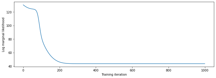
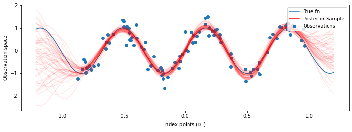
यहां हम एक शोर साइनसॉइड से प्रशिक्षण डेटा उत्पन्न करते हैं, फिर जीपी प्रतिगमन मॉडल के पीछे से वक्रों के एक समूह का नमूना लेते हैं। हम का उपयोग एडम गिरी hyperparameters (हम पहले के तहत डेटा के नकारात्मक लॉग संभावना को कम) अनुकूलन करने के लिए। हम प्रशिक्षण वक्र की साजिश रचते हैं, उसके बाद सही कार्य और पीछे के नमूने।
def sinusoid(x):
  return np.sin(3 * np.pi * x[..., 0])

def generate_1d_data(num_training_points, observation_noise_variance):
  """Generate noisy sinusoidal observations at a random set of points.

  Returns:
     observation_index_points, observations
  """
  index_points_ = np.random.uniform(-1., 1., (num_training_points, 1))
  index_points_ = index_points_.astype(np.float64)
  # y = f(x) + noise
  observations_ = (sinusoid(index_points_) +
                   np.random.normal(loc=0,
                                    scale=np.sqrt(observation_noise_variance),
                                    size=(num_training_points)))
  return index_points_, observations_
# Generate training data with a known noise level (we'll later try to recover
# this value from the data).
NUM_TRAINING_POINTS = 100
observation_index_points_, observations_ = generate_1d_data(
    num_training_points=NUM_TRAINING_POINTS,
    observation_noise_variance=.1)
हम गिरी hyperparameters पर महंतों रखा, और hyperparameters और देखे गए डेटा का उपयोग कर के संयुक्त वितरण लिखेंगे tfd.JointDistributionNamed ।
def build_gp(amplitude, length_scale, observation_noise_variance):
  """Defines the conditional dist. of GP outputs, given kernel parameters."""

  # Create the covariance kernel, which will be shared between the prior (which we
  # use for maximum likelihood training) and the posterior (which we use for
  # posterior predictive sampling)
  kernel = tfk.ExponentiatedQuadratic(amplitude, length_scale)

  # Create the GP prior distribution, which we will use to train the model
  # parameters.
  return tfd.GaussianProcess(
      kernel=kernel,
      index_points=observation_index_points_,
      observation_noise_variance=observation_noise_variance)

gp_joint_model = tfd.JointDistributionNamed({
    'amplitude': tfd.LogNormal(loc=0., scale=np.float64(1.)),
    'length_scale': tfd.LogNormal(loc=0., scale=np.float64(1.)),
    'observation_noise_variance': tfd.LogNormal(loc=0., scale=np.float64(1.)),
    'observations': build_gp,
})
हम यह सत्यापित करके अपने कार्यान्वयन की विवेक-जांच कर सकते हैं कि हम पहले से नमूना ले सकते हैं, और नमूने की लॉग-घनत्व की गणना कर सकते हैं।
x = gp_joint_model.sample()
lp = gp_joint_model.log_prob(x)

print("sampled {}".format(x))
print("log_prob of sample: {}".format(lp))
sampled {'observation_noise_variance': <tf.Tensor: shape=(), dtype=float64, numpy=2.067952217184325>, 'length_scale': <tf.Tensor: shape=(), dtype=float64, numpy=1.154435715487831>, 'amplitude': <tf.Tensor: shape=(), dtype=float64, numpy=5.383850737703549>, 'observations': <tf.Tensor: shape=(100,), dtype=float64, numpy=
array([-2.37070577, -2.05363838, -0.95152824,  3.73509388, -0.2912646 ,
        0.46112342, -1.98018513, -2.10295857, -1.33589756, -2.23027226,
       -2.25081374, -0.89450835, -2.54196452,  1.46621647,  2.32016193,
        5.82399989,  2.27241034, -0.67523432, -1.89150197, -1.39834474,
       -2.33954116,  0.7785609 , -1.42763627, -0.57389025, -0.18226098,
       -3.45098732,  0.27986652, -3.64532398, -1.28635204, -2.42362875,
        0.01107288, -2.53222176, -2.0886136 , -5.54047694, -2.18389607,
       -1.11665628, -3.07161217, -2.06070336, -0.84464262,  1.29238438,
       -0.64973999, -2.63805504, -3.93317576,  0.65546645,  2.24721181,
       -0.73403676,  5.31628298, -1.2208384 ,  4.77782252, -1.42978168,
       -3.3089274 ,  3.25370494,  3.02117591, -1.54862932, -1.07360811,
        1.2004856 , -4.3017773 , -4.95787789, -1.95245901, -2.15960839,
       -3.78592731, -1.74096185,  3.54891595,  0.56294143,  1.15288455,
       -0.77323696,  2.34430694, -1.05302007, -0.7514684 , -0.98321063,
       -3.01300144, -3.00033274,  0.44200837,  0.45060886, -1.84497318,
       -1.89616746, -2.15647664, -2.65672581, -3.65493379,  1.70923375,
       -3.88695218, -0.05151283,  4.51906677, -2.28117003,  3.03032793,
       -1.47713194, -0.35625273,  3.73501587, -2.09328047, -0.60665614,
       -0.78177188, -0.67298545,  2.97436033, -0.29407932,  2.98482427,
       -1.54951178,  2.79206821,  4.2225733 ,  2.56265198,  2.80373284])>}
log_prob of sample: -194.96442183797524
आइए अब उच्चतम पश्च प्रायिकता वाले पैरामीटर मानों को खोजने के लिए अनुकूलित करें। हम प्रत्येक पैरामीटर के लिए एक चर परिभाषित करेंगे, और उनके मानों को सकारात्मक होने के लिए बाध्य करेंगे।
# Create the trainable model parameters, which we'll subsequently optimize.
# Note that we constrain them to be strictly positive.

constrain_positive = tfb.Shift(np.finfo(np.float64).tiny)(tfb.Exp())

amplitude_var = tfp.util.TransformedVariable(
    initial_value=1.,
    bijector=constrain_positive,
    name='amplitude',
    dtype=np.float64)

length_scale_var = tfp.util.TransformedVariable(
    initial_value=1.,
    bijector=constrain_positive,
    name='length_scale',
    dtype=np.float64)

observation_noise_variance_var = tfp.util.TransformedVariable(
    initial_value=1.,
    bijector=constrain_positive,
    name='observation_noise_variance_var',
    dtype=np.float64)

trainable_variables = [v.trainable_variables[0] for v in
                       [amplitude_var,
                       length_scale_var,
                       observation_noise_variance_var]]
हमारे मनाया डेटा पर मॉडल हालत के लिए, हम एक को परिभाषित करेंगे target_log_prob समारोह है, जो (अभी भी अनुमान लगाया जा करने के लिए) कर्नेल hyperparameters लेता है।
def target_log_prob(amplitude, length_scale, observation_noise_variance):
  return gp_joint_model.log_prob({
      'amplitude': amplitude,
      'length_scale': length_scale,
      'observation_noise_variance': observation_noise_variance,
      'observations': observations_
  })
# Now we optimize the model parameters.
num_iters = 1000
optimizer = tf.optimizers.Adam(learning_rate=.01)

# Use `tf.function` to trace the loss for more efficient evaluation.
@tf.function(autograph=False, jit_compile=False)
def train_model():
  with tf.GradientTape() as tape:
    loss = -target_log_prob(amplitude_var, length_scale_var,
                            observation_noise_variance_var)
  grads = tape.gradient(loss, trainable_variables)
  optimizer.apply_gradients(zip(grads, trainable_variables))
  return loss

# Store the likelihood values during training, so we can plot the progress
lls_ = np.zeros(num_iters, np.float64)
for i in range(num_iters):
  loss = train_model()
  lls_[i] = loss

print('Trained parameters:')
print('amplitude: {}'.format(amplitude_var._value().numpy()))
print('length_scale: {}'.format(length_scale_var._value().numpy()))
print('observation_noise_variance: {}'.format(observation_noise_variance_var._value().numpy()))
Trained parameters:
amplitude: 0.9176153445125278
length_scale: 0.18444082442910079
observation_noise_variance: 0.0880273312850989
# Plot the loss evolution
plt.figure(figsize=(12, 4))
plt.plot(lls_)
plt.xlabel("Training iteration")
plt.ylabel("Log marginal likelihood")
plt.show()
# Having trained the model, we'd like to sample from the posterior conditioned
# on observations. We'd like the samples to be at points other than the training
# inputs.
predictive_index_points_ = np.linspace(-1.2, 1.2, 200, dtype=np.float64)
# Reshape to [200, 1] -- 1 is the dimensionality of the feature space.
predictive_index_points_ = predictive_index_points_[..., np.newaxis]

optimized_kernel = tfk.ExponentiatedQuadratic(amplitude_var, length_scale_var)
gprm = tfd.GaussianProcessRegressionModel(
    kernel=optimized_kernel,
    index_points=predictive_index_points_,
    observation_index_points=observation_index_points_,
    observations=observations_,
    observation_noise_variance=observation_noise_variance_var,
    predictive_noise_variance=0.)

# Create op to draw  50 independent samples, each of which is a *joint* draw
# from the posterior at the predictive_index_points_. Since we have 200 input
# locations as defined above, this posterior distribution over corresponding
# function values is a 200-dimensional multivariate Gaussian distribution!
num_samples = 50
samples = gprm.sample(num_samples)
# Plot the true function, observations, and posterior samples.
plt.figure(figsize=(12, 4))
plt.plot(predictive_index_points_, sinusoid(predictive_index_points_),
         label='True fn')
plt.scatter(observation_index_points_[:, 0], observations_,
            label='Observations')
for i in range(num_samples):
  plt.plot(predictive_index_points_, samples[i, :], c='r', alpha=.1,
           label='Posterior Sample' if i == 0 else None)
leg = plt.legend(loc='upper right')
for lh in leg.legendHandles:
    lh.set_alpha(1)
plt.xlabel(r"Index points ($\mathbb{R}^1$)")
plt.ylabel("Observation space")
plt.show()
एचएमसी के साथ हाइपरपैरामीटर को हाशिए पर रखना
हाइपरपैरामीटर को अनुकूलित करने के बजाय, आइए उन्हें हैमिल्टनियन मोंटे कार्लो के साथ एकीकृत करने का प्रयास करें। प्रेक्षणों को देखते हुए, हम पहले कर्नेल हाइपरपैरामीटर पर पश्च वितरण से लगभग ड्रा करने के लिए एक नमूना को परिभाषित और चलाएंगे।
num_results = 100
num_burnin_steps = 50

sampler = tfp.mcmc.TransformedTransitionKernel(
    tfp.mcmc.NoUTurnSampler(
        target_log_prob_fn=target_log_prob,
        step_size=tf.cast(0.1, tf.float64)),
    bijector=[constrain_positive, constrain_positive, constrain_positive])

adaptive_sampler = tfp.mcmc.DualAveragingStepSizeAdaptation(
    inner_kernel=sampler,
    num_adaptation_steps=int(0.8 * num_burnin_steps),
    target_accept_prob=tf.cast(0.75, tf.float64))

initial_state = [tf.cast(x, tf.float64) for x in [1., 1., 1.]]
# Speed up sampling by tracing with `tf.function`.
@tf.function(autograph=False, jit_compile=False)
def do_sampling():
  return tfp.mcmc.sample_chain(
      kernel=adaptive_sampler,
      current_state=initial_state,
      num_results=num_results,
      num_burnin_steps=num_burnin_steps,
      trace_fn=lambda current_state, kernel_results: kernel_results)

t0 = time.time()
samples, kernel_results = do_sampling()
t1 = time.time()
print("Inference ran in {:.2f}s.".format(t1-t0))
Inference ran in 9.00s.
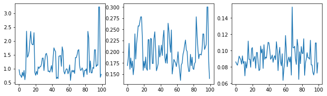
आइए हाइपरपैरामीटर के निशानों की जांच करके सैंपलर की जांच करें।
(amplitude_samples,
 length_scale_samples,
 observation_noise_variance_samples) = samples

f = plt.figure(figsize=[15, 3])
for i, s in enumerate(samples):
  ax = f.add_subplot(1, len(samples) + 1, i + 1)
  ax.plot(s)
अब बजाय अनुकूलित hyperparameters के साथ एक एकल जीपी के निर्माण की है, हम जीपी का मिश्रण है, प्रत्येक hyperparameters से अधिक पिछला वितरण से एक नमूना द्वारा परिभाषित के रूप में पीछे भविष्य कहनेवाला वितरण का निर्माण। यह लगभग मोंटे कार्लो सैंपलिंग के माध्यम से पश्चवर्ती मापदंडों पर एकीकृत होता है, ताकि अनदेखे स्थानों पर सीमांत भविष्य कहनेवाला वितरण की गणना की जा सके।
# The sampled hyperparams have a leading batch dimension, `[num_results, ...]`,
# so they construct a *batch* of kernels.
batch_of_posterior_kernels = tfk.ExponentiatedQuadratic(
    amplitude_samples, length_scale_samples)

# The batch of kernels creates a batch of GP predictive models, one for each
# posterior sample.
batch_gprm = tfd.GaussianProcessRegressionModel(
    kernel=batch_of_posterior_kernels,
    index_points=predictive_index_points_,
    observation_index_points=observation_index_points_,
    observations=observations_,
    observation_noise_variance=observation_noise_variance_samples,
    predictive_noise_variance=0.)

# To construct the marginal predictive distribution, we average with uniform
# weight over the posterior samples.
predictive_gprm = tfd.MixtureSameFamily(
    mixture_distribution=tfd.Categorical(logits=tf.zeros([num_results])),
    components_distribution=batch_gprm)

num_samples = 50
samples = predictive_gprm.sample(num_samples)
# Plot the true function, observations, and posterior samples.
plt.figure(figsize=(12, 4))
plt.plot(predictive_index_points_, sinusoid(predictive_index_points_),
         label='True fn')
plt.scatter(observation_index_points_[:, 0], observations_,
            label='Observations')
for i in range(num_samples):
  plt.plot(predictive_index_points_, samples[i, :], c='r', alpha=.1,
           label='Posterior Sample' if i == 0 else None)
leg = plt.legend(loc='upper right')
for lh in leg.legendHandles:
    lh.set_alpha(1)
plt.xlabel(r"Index points ($\mathbb{R}^1$)")
plt.ylabel("Observation space")
plt.show()
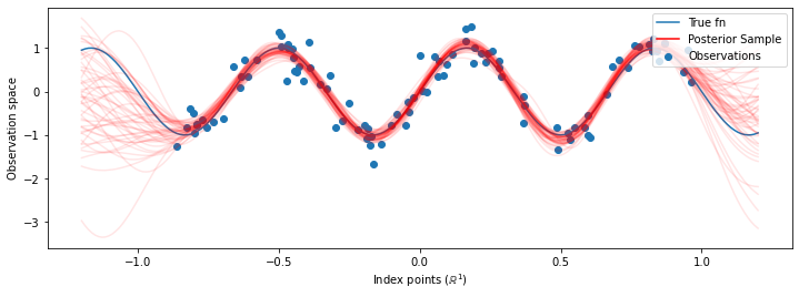
हालांकि इस मामले में अंतर सूक्ष्म हैं, सामान्य तौर पर, हम उम्मीद करेंगे कि पोस्टीरियर प्रेडिक्टिव डिस्ट्रीब्यूशन बेहतर तरीके से सामान्यीकृत होगा (होल्ड-आउट डेटा को उच्च संभावना दें) जैसा कि हमने ऊपर किया था, सबसे संभावित मापदंडों का उपयोग करने की तुलना में।