
| | |  GitHub에서 소스 보기 GitHub에서 소스 보기 | |
TensorFlow 확률 (TFP)은 이제 작동 확률 적 추론 및 통계 분석을위한 라이브러리입니다 JAX ! 익숙하지 않은 사람들을 위해 JAX는 구성 가능한 함수 변환을 기반으로 하는 가속화된 수치 컴퓨팅을 위한 라이브러리입니다.
JAX의 TFP는 많은 TFP 사용자가 현재 편안하게 느끼는 추상화 및 API를 유지하면서 일반 TFP의 가장 유용한 기능을 많이 지원합니다.
설정
JAX에 TFP는 TensorFlow에 의존하지 않는다; 이 Colab에서 TensorFlow를 완전히 제거하겠습니다.
pip uninstall tensorflow -y -q
TFP의 최신 야간 빌드를 사용하여 JAX에 TFP를 설치할 수 있습니다.
pip install -Uq tfp-nightly[jax] > /dev/null
유용한 Python 라이브러리를 가져와 보겠습니다.
import matplotlib.pyplot as plt
import numpy as np
import seaborn as sns
from sklearn import datasets
sns.set(style='white')
/usr/local/lib/python3.6/dist-packages/statsmodels/tools/_testing.py:19: FutureWarning: pandas.util.testing is deprecated. Use the functions in the public API at pandas.testing instead.
  import pandas.util.testing as tm
또한 몇 가지 기본 JAX 기능을 가져오겠습니다.
import jax.numpy as jnp
from jax import grad
from jax import jit
from jax import random
from jax import value_and_grad
from jax import vmap
JAX에서 TFP 가져오기
JAX에 TFP를 사용하려면, 단순히 가져 jax "기판"당신이 일반적으로하는 것처럼 사용 tfp :
from tensorflow_probability.substrates import jax as tfp
tfd = tfp.distributions
tfb = tfp.bijectors
tfpk = tfp.math.psd_kernels
데모: 베이지안 로지스틱 회귀
JAX 백엔드로 무엇을 할 수 있는지 보여주기 위해 클래식 Iris 데이터 세트에 적용된 베이지안 로지스틱 회귀를 구현합니다.
먼저 Iris 데이터세트를 가져오고 일부 메타데이터를 추출해 보겠습니다.
iris = datasets.load_iris()
features, labels = iris['data'], iris['target']

num_features = features.shape[-1]
num_classes = len(iris.target_names)
우리는 사용하여 모델을 정의 할 수 있습니다 tfd.JointDistributionCoroutine . 우리는 다음 쓰기 가중치 및 바이어스 기간 모두에서 표준 정규 전과를 올려 놓을 게요 target_log_prob 기능을하는 핀 데이터에 샘플링 된 레이블.
Root = tfd.JointDistributionCoroutine.Root
def model():
  w = yield Root(tfd.Sample(tfd.Normal(0., 1.),
                            sample_shape=(num_features, num_classes)))
  b = yield Root(
      tfd.Sample(tfd.Normal(0., 1.), sample_shape=(num_classes,)))
  logits = jnp.dot(features, w) + b
  yield tfd.Independent(tfd.Categorical(logits=logits),
                        reinterpreted_batch_ndims=1)


dist = tfd.JointDistributionCoroutine(model)
def target_log_prob(*params):
  return dist.log_prob(params + (labels,))
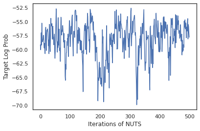
우리는에서 샘플 dist MCMC에 대한 초기 상태를 생성 할 수 있습니다. 그런 다음 임의의 키와 초기 상태를 취하고 No-U-Turn-Sampler(NUTS)에서 500개의 샘플을 생성하는 함수를 정의할 수 있습니다. 우리는 같은 JAX 변환을 사용할 수 있습니다 jit XLA를 사용하여 우리의 너트 샘플러를 컴파일 할 수 있습니다.
init_key, sample_key = random.split(random.PRNGKey(0))
init_params = tuple(dist.sample(seed=init_key)[:-1])

@jit
def run_chain(key, state):
  kernel = tfp.mcmc.NoUTurnSampler(target_log_prob, 1e-3)
  return tfp.mcmc.sample_chain(500,
      current_state=state,
      kernel=kernel,
      trace_fn=lambda _, results: results.target_log_prob,
      num_burnin_steps=500,
      seed=key)

states, log_probs = run_chain(sample_key, init_params)
plt.figure()
plt.plot(log_probs)
plt.ylabel('Target Log Prob')
plt.xlabel('Iterations of NUTS')
plt.show()
샘플을 사용하여 각 가중치 세트의 예측 확률을 평균화하여 베이지안 모델 평균화(BMA)를 수행해 보겠습니다.
먼저 주어진 매개변수 세트에 대해 각 클래스에 대한 확률을 생성하는 함수를 작성해 보겠습니다. 우리는 사용할 수 dist.sample_distributions 모델에 최종 분포를 얻을 수 있습니다.
def classifier_probs(params):
  dists, _ = dist.sample_distributions(seed=random.PRNGKey(0),
                                       value=params + (None,))
  return dists[-1].distribution.probs_parameter()
우리는 할 수 있습니다 vmap(classifier_probs) 우리의 각 시료의 예상 수준의 확률을 얻기 위해 샘플의 집합에. 그런 다음 각 샘플의 평균 정확도와 베이지안 모델 평균화의 정확도를 계산합니다.
all_probs = jit(vmap(classifier_probs))(states)
print('Average accuracy:', jnp.mean(all_probs.argmax(axis=-1) == labels))
print('BMA accuracy:', jnp.mean(all_probs.mean(axis=0).argmax(axis=-1) == labels))
Average accuracy: 0.96952
BMA accuracy: 0.97999996
BMA가 오류율을 거의 1/3로 줄이는 것 같습니다!
기초
JAX에 TFP 대신 TF 객체를 받아들이는 것처럼 TF에 동일한 API가 tf.Tensor 는 JAX 아날로그를 받아들. 예를 들어, 목적지 tf.Tensor 이전에 입력으로 사용하고, API는 현재 JAX 기대 DeviceArray . 대신에 반환하는 tf.Tensor , TFP 방법은 반환 DeviceArray 들. JAX에 TFP는 목록이나 사전 같은 JAX 객체의 중첩 된 구조, 작동 DeviceArray 의.
분포
대부분의 TFP 배포판은 TF 대응물과 매우 유사한 의미로 JAX에서 지원됩니다. 그들은 또한로 등록 JAX Pytrees 들이 JAX 변환 된 함수의 입출력을 할 수 있도록.
기본 배포판
log_prob 분포에 대한 방법은 동일하게 작동합니다.
dist = tfd.Normal(0., 1.)
print(dist.log_prob(0.))
-0.9189385
분포에서 샘플링 명시 적으로 전달해야합니다 PRNGKey 는 AS (또는 정수의 목록) seed 키워드 인수. 명시적으로 시드를 전달하지 않으면 오류가 발생합니다.
tfd.Normal(0., 1.).sample(seed=random.PRNGKey(0))
DeviceArray(-0.20584226, dtype=float32)
분포의 형상의 의미는 각 분포는 것이다 JAX에서 동일하게 유지 event_shape 및 batch_shape 추가 추가되고 드로잉 많은 샘플 sample_shape 크기.
예를 들어, tfd.MultivariateNormalDiag 벡터 매개 변수는 벡터 이벤트 모양과 빈 배치 형태를 가질 것이다.
dist = tfd.MultivariateNormalDiag(
    loc=jnp.zeros(5),
    scale_diag=jnp.ones(5)
)
print('Event shape:', dist.event_shape)
print('Batch shape:', dist.batch_shape)
Event shape: (5,)
Batch shape: ()
한편, tfd.Normal 스칼라 이벤트 형태 및 벡터 배치 형태를 가질 것이다 벡터와 파라미터.
dist = tfd.Normal(
    loc=jnp.ones(5),
    scale=jnp.ones(5),
)
print('Event shape:', dist.event_shape)
print('Batch shape:', dist.batch_shape)
Event shape: ()
Batch shape: (5,)
복용의 의미 log_prob 샘플도 JAX에서 동일하게 작동합니다.
dist =  tfd.Normal(jnp.zeros(5), jnp.ones(5))
s = dist.sample(sample_shape=(10, 2), seed=random.PRNGKey(0))
print(dist.log_prob(s).shape)

dist =  tfd.Independent(tfd.Normal(jnp.zeros(5), jnp.ones(5)), 1)
s = dist.sample(sample_shape=(10, 2), seed=random.PRNGKey(0))
print(dist.log_prob(s).shape)
(10, 2, 5)
(10, 2)
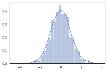
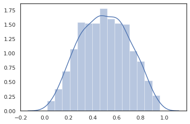
JAX 때문에 DeviceArray s는 NumPy와 및하기 matplotlib 같은 라이브러리와 호환, 우리는 음모를 꾸미고 기능에 직접 샘플을 공급할 수 있습니다.
sns.distplot(tfd.Normal(0., 1.).sample(1000, seed=random.PRNGKey(0)))
plt.show()
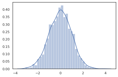
Distribution 방법은 JAX 변환과 호환됩니다.
sns.distplot(jit(vmap(lambda key: tfd.Normal(0., 1.).sample(seed=key)))(
    random.split(random.PRNGKey(0), 2000)))
plt.show()
x = jnp.linspace(-5., 5., 100)
plt.plot(x, jit(vmap(grad(tfd.Normal(0., 1.).prob)))(x))
plt.show()
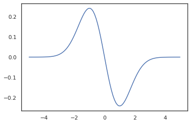
TFP 분포가 JAX의 pytree 노드로 등록되어 있기 때문에, 우리는 입력 또는 출력으로 분포와 함수를 작성하고 사용하여 변환 할 수 jit 하지만 아직 인수로 지원되지 않습니다 vmap -ed 기능을.
@jit
def random_distribution(key):
  loc_key, scale_key = random.split(key)
  loc, log_scale = random.normal(loc_key), random.normal(scale_key)
  return tfd.Normal(loc, jnp.exp(log_scale))
random_dist = random_distribution(random.PRNGKey(0))
print(random_dist.mean(), random_dist.variance())
0.14389051 0.081832744
변환된 분포
변형 된 배포판은 누구를 샘플링 통과 분포, 즉 Bijector 또한 상자의 운동 (bijectors도 작동! 아래 참조).
dist = tfd.TransformedDistribution(
    tfd.Normal(0., 1.),
    tfb.Sigmoid()
)
sns.distplot(dist.sample(1000, seed=random.PRNGKey(0)))
plt.show()
공동 분포
TFP는 제공 JointDistribution 의 여러 확률 변수 위에 단일 분포로 성분 분포들을 조합 활성화한다. 현재 TFP 제공 세 가지 핵심 변종 ( JointDistributionSequential , JointDistributionNamed 및 JointDistributionCoroutine ) 모두 JAX에서 지원됩니다. AutoBatched 변종은 모두 지원됩니다.
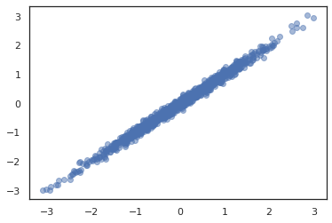
dist = tfd.JointDistributionSequential([
  tfd.Normal(0., 1.),
  lambda x: tfd.Normal(x, 1e-1)
])
plt.scatter(*dist.sample(1000, seed=random.PRNGKey(0)), alpha=0.5)
plt.show()
joint = tfd.JointDistributionNamed(dict(
    e=             tfd.Exponential(rate=1.),
    n=             tfd.Normal(loc=0., scale=2.),
    m=lambda n, e: tfd.Normal(loc=n, scale=e),
    x=lambda    m: tfd.Sample(tfd.Bernoulli(logits=m), 12),
))
joint.sample(seed=random.PRNGKey(0))
{'e': DeviceArray(3.376818, dtype=float32),
 'm': DeviceArray(2.5449684, dtype=float32),
 'n': DeviceArray(-0.6027825, dtype=float32),
 'x': DeviceArray([1, 1, 1, 1, 1, 1, 1, 1, 1, 1, 1, 1], dtype=int32)}
Root = tfd.JointDistributionCoroutine.Root
def model():
  e = yield Root(tfd.Exponential(rate=1.))
  n = yield Root(tfd.Normal(loc=0, scale=2.))
  m = yield tfd.Normal(loc=n, scale=e)
  x = yield tfd.Sample(tfd.Bernoulli(logits=m), 12)

joint = tfd.JointDistributionCoroutine(model)

joint.sample(seed=random.PRNGKey(0))
StructTuple(var0=DeviceArray(0.17315261, dtype=float32), var1=DeviceArray(-3.290489, dtype=float32), var2=DeviceArray(-3.1949058, dtype=float32), var3=DeviceArray([0, 0, 0, 0, 0, 0, 0, 0, 0, 0, 0, 0], dtype=int32))
기타 배포판
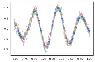
가우스 프로세스는 JAX 모드에서도 작동합니다!
k1, k2, k3 = random.split(random.PRNGKey(0), 3)
observation_noise_variance = 0.01
f = lambda x: jnp.sin(10*x[..., 0]) * jnp.exp(-x[..., 0]**2)
observation_index_points = random.uniform(
    k1, [50], minval=-1.,maxval= 1.)[..., jnp.newaxis]
observations = f(observation_index_points) + tfd.Normal(
    loc=0., scale=jnp.sqrt(observation_noise_variance)).sample(seed=k2)

index_points = jnp.linspace(-1., 1., 100)[..., jnp.newaxis]

kernel = tfpk.ExponentiatedQuadratic(length_scale=0.1)

gprm = tfd.GaussianProcessRegressionModel(
    kernel=kernel,
    index_points=index_points,
    observation_index_points=observation_index_points,
    observations=observations,
    observation_noise_variance=observation_noise_variance)

samples = gprm.sample(10, seed=k3)
for i in range(10):
  plt.plot(index_points, samples[i], alpha=0.5)
plt.plot(observation_index_points, observations, marker='o', linestyle='')
plt.show()
은닉 마르코프 모델도 지원됩니다.
initial_distribution = tfd.Categorical(probs=[0.8, 0.2])
transition_distribution = tfd.Categorical(probs=[[0.7, 0.3],
                                                 [0.2, 0.8]])

observation_distribution = tfd.Normal(loc=[0., 15.], scale=[5., 10.])

model = tfd.HiddenMarkovModel(
    initial_distribution=initial_distribution,
    transition_distribution=transition_distribution,
    observation_distribution=observation_distribution,
    num_steps=7)

print(model.mean())
print(model.log_prob(jnp.zeros(7)))
print(model.sample(seed=random.PRNGKey(0)))
[3.       6.       7.5      8.249999 8.625001 8.812501 8.90625 ]
/usr/local/lib/python3.6/dist-packages/tensorflow_probability/substrates/jax/distributions/hidden_markov_model.py:483: UserWarning: HiddenMarkovModel.log_prob in TFP versions < 0.12.0 had a bug in which the transition model was applied prior to the initial step. This bug has been fixed. You may observe a slight change in behavior.
  'HiddenMarkovModel.log_prob in TFP versions < 0.12.0 had a bug '
-19.855635
[ 1.3641367  0.505798   1.3626463  3.6541772  2.272286  15.10309
 22.794212 ]
같은 몇 분포 PixelCNN 때문에 TensorFlow 또는 XLA 호환성에 대한 엄격한 종속성 아직 지원되지 않습니다.
바이젝터
오늘날 대부분의 TFP 바이젝터는 JAX에서 지원됩니다!
tfb.Exp().inverse(1.)
DeviceArray(0., dtype=float32)
bij = tfb.Shift(1.)(tfb.Scale(3.))
print(bij.forward(jnp.ones(5)))
print(bij.inverse(jnp.ones(5)))
[4. 4. 4. 4. 4.]
[0. 0. 0. 0. 0.]
b = tfb.FillScaleTriL(diag_bijector=tfb.Exp(), diag_shift=None)
print(b.forward(x=[0., 0., 0.]))
print(b.inverse(y=[[1., 0], [.5, 2]]))
[[1. 0.]
 [0. 1.]]
[0.6931472 0.5       0.       ]
b = tfb.Chain([tfb.Exp(), tfb.Softplus()])
# or:
# b = tfb.Exp()(tfb.Softplus())
print(b.forward(-jnp.ones(5)))
[1.3678794 1.3678794 1.3678794 1.3678794 1.3678794]
Bijectors 같은 JAX 변환과 호환되는 jit , grad 및 vmap .
jit(vmap(tfb.Exp().inverse))(jnp.arange(4.))
DeviceArray([ -inf, 0. , 0.6931472, 1.0986123], dtype=float32)
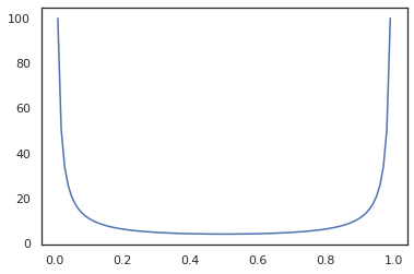
x = jnp.linspace(0., 1., 100)
plt.plot(x, jit(grad(lambda x: vmap(tfb.Sigmoid().inverse)(x).sum()))(x))
plt.show()
같은 일부 bijectors, RealNVP 및 FFJORD 아직 지원되지 않습니다.
MCMC
우리는 포팅했습니다 tfp.mcmc 우리가 해밀턴 몬테 카를로 (HMC) 및 JAX에서 (너트) 없음-U 턴 - 샘플러와 같은 알고리즘을 실행할 수 있도록뿐만 아니라 JAX에.
target_log_prob = tfd.MultivariateNormalDiag(jnp.zeros(2), jnp.ones(2)).log_prob
TF에 TFP는 달리, 우리는 통과해야 PRNGKey 에 sample_chain 은 Using seed 키워드 인수를.
def run_chain(key, state):
kernel = tfp.mcmc.NoUTurnSampler(target_log_prob, 1e-1)
return tfp.mcmc.sample_chain(1000,
current_state=state,
kernel=kernel,
trace_fn=lambda _, results: results.target_log_prob,
seed=key)
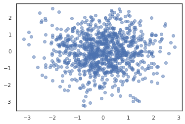
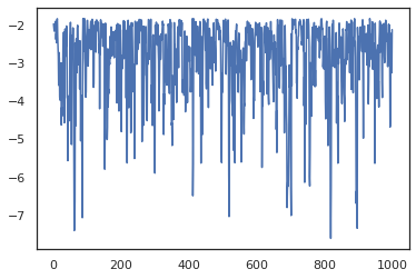
states, log_probs = jit(run_chain)(random.PRNGKey(0), jnp.zeros(2))
plt.figure()
plt.scatter(*states.T, alpha=0.5)
plt.figure()
plt.plot(log_probs)
plt.show()
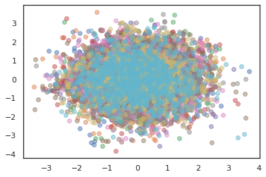
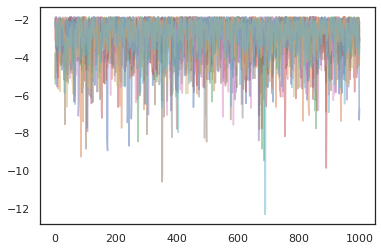
여러 개의 체인을 실행하려면, 우리는 하나에 국가의 배치를 통과 할 수 sample_chain 또는 사용 vmap (우리는 아직 두 가지 방법 사이의 성능 차이를 탐구하지 않은 있지만).
states, log_probs = jit(run_chain)(random.PRNGKey(0), jnp.zeros([10, 2]))
plt.figure()
for i in range(10):
  plt.scatter(*states[:, i].T, alpha=0.5)
plt.figure()
for i in range(10):
  plt.plot(log_probs[:, i], alpha=0.5)
plt.show()
옵티마이저
JAX의 TFP는 BFGS 및 L-BFGS와 같은 몇 가지 중요한 최적화 프로그램을 지원합니다. 간단한 스케일링된 2차 손실 함수를 설정해 보겠습니다.
minimum = jnp.array([1.0, 1.0])  # The center of the quadratic bowl.
scales = jnp.array([2.0, 3.0])  # The scales along the two axes.

# The objective function and the gradient.
def quadratic_loss(x):
  return jnp.sum(scales * jnp.square(x - minimum))

start = jnp.array([0.6, 0.8])  # Starting point for the search.
BFGS는 이 손실의 최소값을 찾을 수 있습니다.
optim_results = tfp.optimizer.bfgs_minimize(
    value_and_grad(quadratic_loss), initial_position=start, tolerance=1e-8)

# Check that the search converged
assert(optim_results.converged)
# Check that the argmin is close to the actual value.
np.testing.assert_allclose(optim_results.position, minimum)
# Print out the total number of function evaluations it took. Should be 5.
print("Function evaluations: %d" % optim_results.num_objective_evaluations)
Function evaluations: 5
L-BFGS도 마찬가지입니다.
optim_results = tfp.optimizer.lbfgs_minimize(
    value_and_grad(quadratic_loss), initial_position=start, tolerance=1e-8)

# Check that the search converged
assert(optim_results.converged)
# Check that the argmin is close to the actual value.
np.testing.assert_allclose(optim_results.position, minimum)
# Print out the total number of function evaluations it took. Should be 5.
print("Function evaluations: %d" % optim_results.num_objective_evaluations)
Function evaluations: 5
하기 vmap L-BFGS을 하나의 출발점에 대한 손실을 최적화하는 기능까지의 설정을 할 수 있습니다.
def optimize_single(start):
  return tfp.optimizer.lbfgs_minimize(
      value_and_grad(quadratic_loss), initial_position=start, tolerance=1e-8)

all_results = jit(vmap(optimize_single))(
    random.normal(random.PRNGKey(0), (10, 2)))
assert all(all_results.converged)
for i in range(10):
  np.testing.assert_allclose(optim_results.position[i], minimum)
print("Function evaluations: %s" % all_results.num_objective_evaluations)
Function evaluations: [6 6 9 6 6 8 6 8 5 9]
주의 사항
TF와 JAX 사이에는 몇 가지 근본적인 차이점이 있으며 일부 TFP 동작은 두 기판 간에 다르며 모든 기능이 지원되는 것은 아닙니다. 예를 들어,
- JAX에 TFP는 같은 것을 지원하지 않습니다
tf.Variable가 JAX 존재처럼 아무것도 때문이다. 이것은 또한 같은 유틸리티 의미tfp.util.TransformedVariable중 하나를 지원하지 않습니다. -
tfp.layers때문에 Keras과에 대한 의존도에, 아직 백엔드에서 지원되지 않습니다tf.Variable의. -
tfp.math.minimize때문에에 대한 의존도의 JAX에 TFP에서 작업을하지 않는tf.Variable. - JAX의 TFP를 사용하면 텐서 모양은 항상 구체적인 정수 값이며 TF의 TFP와 같이 알 수 없거나 동적이지 않습니다.
- 의사 난수는 TF와 JAX에서 다르게 처리됩니다(부록 참조).
- 도서관
tfp.experimental잭스 기판에 존재 보장 할 수 없습니다. - Dtype 승격 규칙은 TF와 JAX 간에 다릅니다. JAX의 TFP는 일관성을 위해 내부적으로 TF의 dtype 의미 체계를 존중하려고 합니다.
- 바이젝터는 아직 JAX 파이트리로 등록되지 않았습니다.
JAX에 TFP에서 지원 무엇의 전체 목록을 보려면를 참조하십시오 API 문서 .
결론
우리는 많은 TFP 기능을 JAX로 이식했으며 모두가 무엇을 빌드할지 기대됩니다. 일부 기능은 아직 지원되지 않습니다. 우리는 당신에게 중요한 것을 놓친 경우 (또는 당신이 버그를 발견하면!) 우리에게 문의하시기 바랍니다 - 당신은 이메일을 보낼 수 tfprobability@tensorflow.org 또는에 문제를 제기 우리 Github에서의 REPO .
부록: JAX의 의사 난수
JAX의 의사 난수 생성 (PRNG) 모델은 비 상태입니다. 상태 저장 모델과 달리 각 무작위 추첨 후에 진화하는 변경 가능한 전역 상태가 없습니다. JAX의 모델에서, 우리는 32 비트 정수의 쌍과 같은 역할을하는 PRNG 키를 시작합니다. 우리는 사용하여 이러한 키를 생성 할 수 있습니다 jax.random.PRNGKey .
key = random.PRNGKey(0)  # Creates a key with value [0, 0]
print(key)
[0 0]
결정적으로 그들이 다시 사용할 수 없습니다 의미, 임의의 변량 생산에 JAX에서 임의의 기능 키를 소비한다. 예를 들어, 우리가 사용할 수있는 key 정상적으로 분산 값을 샘플링 할 수 있지만, 우리는 사용하지 말아야 key 를 다시 다른 곳에서. 더욱이, 동일한 값으로 전달 random.normal 동일한 값을 생성한다.
print(random.normal(key))
-0.20584226
그렇다면 단일 키에서 어떻게 여러 샘플을 그릴 수 있습니까? 대답은 키 분할이다. 기본적인 아이디어는 우리가 나눌 수 있다는 것입니다 PRNGKey 복수로, 새로운 각각의 키는 난수의 독립적 인 소스로 처리 할 수있다.
key1, key2 = random.split(key, num=2)
print(key1, key2)
[4146024105 967050713] [2718843009 1272950319]
키 분할은 결정적이지만 혼란스럽기 때문에 이제 각각의 새 키를 사용하여 고유한 무작위 샘플을 그릴 수 있습니다.
print(random.normal(key1), random.normal(key2))
0.14389051 -1.2515389
JAX의 결정적 키 분할 모델에 대한 자세한 내용은 볼 이 가이드를 .