| | |  Lihat sumber di GitHub Lihat sumber di GitHub | |
Ini adalah port Probabilitas TensorFlow dari makalah 16 Maret 2020 eponymous oleh Li et al. Kami dengan setia mereproduksi metode dan hasil penulis asli di platform TensorFlow Probability, menampilkan beberapa kemampuan TFP dalam pengaturan pemodelan epidemiologi modern. Porting ke TensorFlow memberi kami kecepatan ~10x relatif terhadap kode Matlab asli, dan, karena TensorFlow Probability secara luas mendukung komputasi batch yang di-vektor, juga menskalakan dengan baik hingga ratusan replikasi independen.
kertas asli
Ruiyun Li, Sen Pei, Bin Chen, Lagu Yimeng, Tao Zhang, Wan Yang, dan Jeffrey Shaman. Infeksi substansial yang tidak terdokumentasi memfasilitasi penyebaran cepat virus corona baru (SARS-CoV2). (2020), doi: https://doi.org/10.1126/science.abb3221 .
Abstrak:. "Estimasi prevalensi dan Penularan novel coronavirus (SARS-CoV2) infeksi tak tercatat sangat penting untuk memahami prevalensi keseluruhan dan potensi pandemi penyakit ini Di sini kita menggunakan pengamatan infeksi dilaporkan di China, dalam hubungannya dengan data mobilitas, sebuah model metapopulasi dinamis jaringan dan inferensi Bayesian, untuk menyimpulkan karakteristik epidemiologi kritis yang terkait dengan SARS-CoV2, termasuk fraksi infeksi yang tidak terdokumentasi dan penularannya. Kami memperkirakan 86% dari semua infeksi tidak terdokumentasi (95% CI: [82% -90%] ) sebelum pembatasan perjalanan 23 Januari 2020. Per orang, tingkat penularan infeksi tidak berdokumen adalah 55% dari infeksi yang terdokumentasi ([46% –62%), namun, karena jumlahnya yang lebih besar, infeksi tidak berdokumen adalah sumber infeksi untuk 79 % dari kasus yang terdokumentasi. Temuan ini menjelaskan penyebaran geografis yang cepat dari SARS-CoV2 dan menunjukkan penahanan virus ini akan sangat menantang."
Github menghubungkan ke kode dan data.
Ringkasan
Model ini merupakan model yang penyakit kompartemen , dengan kompartemen untuk "rentan", "terkena" (terinfeksi tetapi belum menular), "tidak pernah didokumentasikan menular", dan "akhirnya didokumentasikan menular". Ada dua fitur penting: kompartemen terpisah untuk masing-masing dari 375 kota di Cina, dengan asumsi tentang bagaimana orang bepergian dari satu kota ke kota lain; dan keterlambatan dalam pelaporan infeksi, sehingga kasus yang menjadi "akhirnya didokumentasikan menular" pada hari \(t\) tidak muncul dalam jumlah kasus yang diamati sampai hari kemudian stokastik.
Model tersebut mengasumsikan bahwa kasus-kasus yang tidak pernah terdokumentasikan menjadi tidak terdokumentasi karena lebih ringan, dan dengan demikian menginfeksi orang lain pada tingkat yang lebih rendah. Parameter utama yang menarik dalam makalah asli adalah proporsi kasus yang tidak terdokumentasi, untuk memperkirakan tingkat infeksi yang ada, dan dampak penularan tidak berdokumen pada penyebaran penyakit.
Colab ini disusun sebagai panduan kode dalam gaya bottom-up. Secara berurutan, kami akan
- Mencerna dan memeriksa data secara singkat,
- Tentukan ruang keadaan dan dinamika model,
- Bangun serangkaian fungsi untuk melakukan inferensi dalam model berikut Li et al, dan
- Panggil mereka dan periksa hasilnya. Spoiler: Mereka keluar sama seperti kertas.
Instalasi dan Impor Python
pip3 install -q tf-nightly tfp-nightly
import collections
import io
import requests
import time
import zipfile

import matplotlib.pyplot as plt
import numpy as np
import pandas as pd

import tensorflow.compat.v2 as tf
import tensorflow_probability as tfp
from tensorflow_probability.python.internal import samplers

tfd = tfp.distributions
tfes = tfp.experimental.sequential
Impor Data
Mari impor data dari github dan periksa sebagian.
r = requests.get('https://raw.githubusercontent.com/SenPei-CU/COVID-19/master/Data.zip')
z = zipfile.ZipFile(io.BytesIO(r.content))
z.extractall('/tmp/')
raw_incidence = pd.read_csv('/tmp/data/Incidence.csv')
raw_mobility = pd.read_csv('/tmp/data/Mobility.csv')
raw_population = pd.read_csv('/tmp/data/pop.csv')
Di bawah ini kita dapat melihat jumlah kejadian mentah per hari. Kami paling tertarik pada 14 hari pertama (10 Januari hingga 23 Januari), karena pembatasan perjalanan diberlakukan pada tanggal 23. Makalah ini membahas hal ini dengan memodelkan 10-23 Januari dan 23 Januari+ secara terpisah, dengan parameter yang berbeda; kita hanya akan membatasi reproduksi kita pada periode sebelumnya.
raw_incidence.drop('Date', axis=1)  # The 'Date' column is all 1/18/21
# Luckily the days are in order, starting on January 10th, 2020.
Mari kita periksa kewarasan jumlah insiden di Wuhan.
plt.plot(raw_incidence.Wuhan, '.-')
plt.title('Wuhan incidence counts over 1/10/20 - 02/08/20')
plt.show()
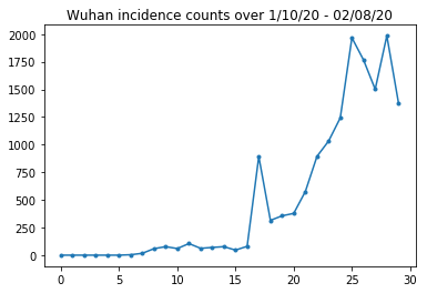
Sejauh ini bagus. Sekarang jumlah populasi awal.
raw_population
Mari kita periksa juga dan catat entri mana yang merupakan Wuhan.
raw_population['City'][169]
'Wuhan'
WUHAN_IDX = 169
Dan di sini kita melihat matriks mobilitas antar kota yang berbeda. Ini adalah proksi untuk jumlah orang yang berpindah antar kota yang berbeda pada 14 hari pertama. Ini berasal dari catatan GPS yang disediakan oleh Tencent untuk musim Tahun Baru Imlek 2018. Li et al mobilitas Model selama musim 2020 karena beberapa yang tidak diketahui (tunduk inferensi) faktor konstan \(\theta\) kali ini.
raw_mobility
Terakhir, mari kita praproses semua ini menjadi array numpy yang bisa kita konsumsi.
# The given populations are only "initial" because of intercity mobility during
# the holiday season.
initial_population = raw_population['Population'].to_numpy().astype(np.float32)
Ubah data mobilitas menjadi Tensor berbentuk [L, L, T], di mana L adalah jumlah lokasi, dan T adalah jumlah langkah waktu.
daily_mobility_matrices = []
for i in range(1, 15):
  day_mobility = raw_mobility[raw_mobility['Day'] == i]

  # Make a matrix of daily mobilities.
  z = pd.crosstab(
      day_mobility.Origin,
      day_mobility.Destination,
      values=day_mobility['Mobility Index'], aggfunc='sum', dropna=False)

  # Include every city, even if there are no rows for some in the raw data on
  # some day.  This uses the sort order of `raw_population`.
  z = z.reindex(index=raw_population['City'], columns=raw_population['City'],
                fill_value=0)
  # Finally, fill any missing entries with 0. This means no mobility.
  z = z.fillna(0)
  daily_mobility_matrices.append(z.to_numpy())

mobility_matrix_over_time = np.stack(daily_mobility_matrices, axis=-1).astype(
    np.float32)
Akhirnya ambil infeksi yang diamati dan buat tabel [L, T].
# Remove the date parameter and take the first 14 days.
observed_daily_infectious_count = raw_incidence.to_numpy()[:14, 1:]
observed_daily_infectious_count = np.transpose(
    observed_daily_infectious_count).astype(np.float32)
Dan periksa kembali apakah kami mendapatkan bentuk seperti yang kami inginkan. Sebagai pengingat, kami bekerja dengan 375 kota dan 14 hari.
print('Mobility Matrix over time should have shape (375, 375, 14): {}'.format(
    mobility_matrix_over_time.shape))
print('Observed Infectious should have shape (375, 14): {}'.format(
    observed_daily_infectious_count.shape))
print('Initial population should have shape (375): {}'.format(
    initial_population.shape))
Mobility Matrix over time should have shape (375, 375, 14): (375, 375, 14)
Observed Infectious should have shape (375, 14): (375, 14)
Initial population should have shape (375): (375,)
Menentukan Status dan Parameter
Mari kita mulai mendefinisikan model kita. Model kita mereproduksi adalah varian dari model yang Seir . Dalam hal ini kita memiliki status variasi waktu berikut:
- \(S\): Jumlah orang yang rentan terhadap penyakit di setiap kota.
- \(E\): Jumlah orang di setiap kota terkena penyakit tetapi tidak menular belum. Secara biologis, ini sesuai dengan tertular penyakit, di mana semua orang yang terpapar akhirnya menjadi menular.
- \(I^u\): Jumlah orang di setiap kota yang menular tapi tidak tercatat. Dalam model, ini sebenarnya berarti "tidak akan pernah didokumentasikan".
- \(I^r\): Jumlah orang di setiap kota yang menular dan didokumentasikan seperti itu. Li et al Model keterlambatan pelaporan, sehingga \(I^r\) benar-benar sesuai untuk sesuatu seperti "kasus cukup parah untuk didokumentasikan di beberapa titik di masa depan".
Seperti yang akan kita lihat di bawah, kita akan menyimpulkan status ini dengan menjalankan Ensemble-adjusted Kalman Filter (EAKF) ke depan tepat waktu. Vektor keadaan EAKF adalah satu vektor terindeks kota untuk masing-masing besaran ini.
Model ini memiliki parameter invarian global dan invarian waktu berikut:
- \(\beta\): Tingkat transmisi karena individu-menular didokumentasikan.
- \(\mu\): Tingkat transmisi relatif karena individu tidak berdokumen-menular. Hal ini akan bertindak melalui produk \(\mu \beta\).
- \(\theta\): Faktor mobilitas antarkota. Ini adalah faktor yang lebih besar dari 1 koreksi untuk pelaporan data mobilitas yang kurang (dan untuk pertumbuhan populasi dari 2018 hingga 2020).
- \(Z\): Masa inkubasi rata-rata (yaitu, waktu di "terkena" negara).
- \(\alpha\): ini adalah sebagian kecil dari infeksi cukup untuk menjadi berat (akhirnya) didokumentasikan.
- \(D\): Rata-rata durasi infeksi (yaitu, waktu baik "menular" negara).
Kami akan menyimpulkan estimasi titik untuk parameter ini dengan loop Iterative-Filtering di sekitar EAKF untuk negara bagian.
Model juga bergantung pada konstanta yang tidak disimpulkan:
- \(M\): Mobilitas antarkota matriks. Ini adalah waktu yang bervariasi dan dianggap diberikan. Ingat bahwa itu skala oleh disimpulkan parameter \(\theta\) untuk memberikan perpindahan penduduk sebenarnya antara kota.
- \(N\): Jumlah total orang di setiap kota. Populasi awal yang diambil seperti yang diberikan, dan waktu-variasi populasi dihitung dari angka mobilitas \(\theta M\).
Pertama, kami memberi diri kami beberapa struktur data untuk menyimpan status dan parameter kami.
SEIRComponents = collections.namedtuple(
  typename='SEIRComponents',
  field_names=[
    'susceptible',              # S
    'exposed',                  # E
    'documented_infectious',    # I^r
    'undocumented_infectious',  # I^u
    # This is the count of new cases in the "documented infectious" compartment.
    # We need this because we will introduce a reporting delay, between a person
    # entering I^r and showing up in the observable case count data.
    # This can't be computed from the cumulative `documented_infectious` count,
    # because some portion of that population will move to the 'recovered'
    # state, which we aren't tracking explicitly.
    'daily_new_documented_infectious'])

ModelParams = collections.namedtuple(
    typename='ModelParams',
    field_names=[
      'documented_infectious_tx_rate',             # Beta
      'undocumented_infectious_tx_relative_rate',  # Mu
      'intercity_underreporting_factor',           # Theta
      'average_latency_period',                    # Z
      'fraction_of_documented_infections',         # Alpha
      'average_infection_duration'                 # D
    ]
)
Kami juga mengkode batas Li et al untuk nilai parameter.
PARAMETER_LOWER_BOUNDS = ModelParams(
    documented_infectious_tx_rate=0.8,
    undocumented_infectious_tx_relative_rate=0.2,
    intercity_underreporting_factor=1.,
    average_latency_period=2.,
    fraction_of_documented_infections=0.02,
    average_infection_duration=2.
)

PARAMETER_UPPER_BOUNDS = ModelParams(
    documented_infectious_tx_rate=1.5,
    undocumented_infectious_tx_relative_rate=1.,
    intercity_underreporting_factor=1.75,
    average_latency_period=5.,
    fraction_of_documented_infections=1.,
    average_infection_duration=5.
)
Dinamika SEIR
Di sini kita mendefinisikan hubungan antara parameter dan keadaan.
Persamaan dinamika waktu dari Li et al (bahan pelengkap, persamaan 1-5) adalah sebagai berikut:
\(\frac{dS_i}{dt} = -\beta \frac{S_i I_i^r}{N_i} - \mu \beta \frac{S_i I_i^u}{N_i} + \theta \sum_k \frac{M_{ij} S_j}{N_j - I_j^r} - + \theta \sum_k \frac{M_{ji} S_j}{N_i - I_i^r}\)
\(\frac{dE_i}{dt} = \beta \frac{S_i I_i^r}{N_i} + \mu \beta \frac{S_i I_i^u}{N_i} -\frac{E_i}{Z} + \theta \sum_k \frac{M_{ij} E_j}{N_j - I_j^r} - + \theta \sum_k \frac{M_{ji} E_j}{N_i - I_i^r}\)
\(\frac{dI^r_i}{dt} = \alpha \frac{E_i}{Z} - \frac{I_i^r}{D}\)
\(\frac{dI^u_i}{dt} = (1 - \alpha) \frac{E_i}{Z} - \frac{I_i^u}{D} + \theta \sum_k \frac{M_{ij} I_j^u}{N_j - I_j^r} - + \theta \sum_k \frac{M_{ji} I^u_j}{N_i - I_i^r}\)
\(N_i = N_i + \theta \sum_j M_{ij} - \theta \sum_j M_{ji}\)
Sebagai pengingat, para \(i\) dan \(j\) indeks subscript kota. Persamaan ini memodelkan waktu-evolusi penyakit melalui
- Kontak dengan individu yang menular menyebabkan lebih banyak infeksi;
- Perkembangan penyakit dari "terpapar" ke salah satu keadaan "menular";
- Perkembangan penyakit dari keadaan "menular" ke pemulihan, yang kami modelkan dengan menghilangkan populasi yang dimodelkan;
- Mobilitas antar kota, termasuk orang-orang menular yang terpapar atau tidak berdokumen; dan
- Variasi waktu penduduk kota harian melalui mobilitas antar kota.
Mengikuti Li et al, kami berasumsi bahwa orang dengan kasus yang cukup parah untuk akhirnya dilaporkan tidak melakukan perjalanan antar kota.
Juga mengikuti Li et al, kami memperlakukan dinamika ini sebagai subjek dari kebisingan Poisson term-bijaksana, yaitu, setiap suku sebenarnya adalah laju Poisson, sampel yang memberikan perubahan sebenarnya. Kebisingan Poisson bersifat term-bijaksana karena pengurangan (sebagai lawan penambahan) sampel Poisson tidak menghasilkan hasil terdistribusi Poisson.
Kami akan mengembangkan dinamika ini ke depan dalam waktu dengan integrator Runge-Kutta orde keempat klasik, tetapi pertama-tama mari kita definisikan fungsi yang menghitungnya (termasuk pengambilan sampel derau Poisson).
def sample_state_deltas(
    state, population, mobility_matrix, params, seed, is_deterministic=False):
  """Computes one-step change in state, including Poisson sampling.

  Note that this is coded to support vectorized evaluation on arbitrary-shape
  batches of states.  This is useful, for example, for running multiple
  independent replicas of this model to compute credible intervals for the
  parameters.  We refer to the arbitrary batch shape with the conventional
  `B` in the parameter documentation below.  This function also, of course,
  supports broadcasting over the batch shape.

  Args:
    state: A `SEIRComponents` tuple with fields Tensors of shape
      B + [num_locations] giving the current disease state.
    population: A Tensor of shape B + [num_locations] giving the current city
      populations.
    mobility_matrix: A Tensor of shape B + [num_locations, num_locations] giving
      the current baseline inter-city mobility.
    params: A `ModelParams` tuple with fields Tensors of shape B giving the
      global parameters for the current EAKF run.
    seed: Initial entropy for pseudo-random number generation.  The Poisson
      sampling is repeatable by supplying the same seed.
    is_deterministic: A `bool` flag to turn off Poisson sampling if desired.

  Returns:
    delta: A `SEIRComponents` tuple with fields Tensors of shape
      B + [num_locations] giving the one-day changes in the state, according
      to equations 1-4 above (including Poisson noise per Li et al).
  """
  undocumented_infectious_fraction = state.undocumented_infectious / population
  documented_infectious_fraction = state.documented_infectious / population

  # Anyone not documented as infectious is considered mobile
  mobile_population = (population - state.documented_infectious)
  def compute_outflow(compartment_population):
    raw_mobility = tf.linalg.matvec(
        mobility_matrix, compartment_population / mobile_population)
    return params.intercity_underreporting_factor * raw_mobility
  def compute_inflow(compartment_population):
    raw_mobility = tf.linalg.matmul(
        mobility_matrix,
        (compartment_population / mobile_population)[..., tf.newaxis],
        transpose_a=True)
    return params.intercity_underreporting_factor * tf.squeeze(
        raw_mobility, axis=-1)

  # Helper for sampling the Poisson-variate terms.
  seeds = samplers.split_seed(seed, n=11)
  if is_deterministic:
    def sample_poisson(rate):
      return rate
  else:
    def sample_poisson(rate):
      return tfd.Poisson(rate=rate).sample(seed=seeds.pop())

  # Below are the various terms called U1-U12 in the paper. We combined the
  # first two, which should be fine; both are poisson so their sum is too, and
  # there's no risk (as there could be in other terms) of going negative.
  susceptible_becoming_exposed = sample_poisson(
      state.susceptible *
      (params.documented_infectious_tx_rate *
       documented_infectious_fraction +
       (params.undocumented_infectious_tx_relative_rate *
        params.documented_infectious_tx_rate) *
       undocumented_infectious_fraction))  # U1 + U2

  susceptible_population_inflow = sample_poisson(
      compute_inflow(state.susceptible))  # U3
  susceptible_population_outflow = sample_poisson(
      compute_outflow(state.susceptible))  # U4

  exposed_becoming_documented_infectious = sample_poisson(
      params.fraction_of_documented_infections *
      state.exposed / params.average_latency_period)  # U5
  exposed_becoming_undocumented_infectious = sample_poisson(
      (1 - params.fraction_of_documented_infections) *
      state.exposed / params.average_latency_period)  # U6

  exposed_population_inflow = sample_poisson(
      compute_inflow(state.exposed))  # U7
  exposed_population_outflow = sample_poisson(
      compute_outflow(state.exposed))  # U8

  documented_infectious_becoming_recovered = sample_poisson(
      state.documented_infectious /
      params.average_infection_duration)  # U9
  undocumented_infectious_becoming_recovered = sample_poisson(
      state.undocumented_infectious /
      params.average_infection_duration)  # U10

  undocumented_infectious_population_inflow = sample_poisson(
      compute_inflow(state.undocumented_infectious))  # U11
  undocumented_infectious_population_outflow = sample_poisson(
      compute_outflow(state.undocumented_infectious))  # U12

  # The final state_deltas
  return SEIRComponents(
      # Equation [1]
      susceptible=(-susceptible_becoming_exposed +
                   susceptible_population_inflow +
                   -susceptible_population_outflow),
      # Equation [2]
      exposed=(susceptible_becoming_exposed +
               -exposed_becoming_documented_infectious +
               -exposed_becoming_undocumented_infectious +
               exposed_population_inflow +
               -exposed_population_outflow),
      # Equation [3]
      documented_infectious=(
          exposed_becoming_documented_infectious +
          -documented_infectious_becoming_recovered),
      # Equation [4]
      undocumented_infectious=(
          exposed_becoming_undocumented_infectious +
          -undocumented_infectious_becoming_recovered +
          undocumented_infectious_population_inflow +
          -undocumented_infectious_population_outflow),
      # New to-be-documented infectious cases, subject to the delayed
      # observation model.
      daily_new_documented_infectious=exposed_becoming_documented_infectious)
Berikut integratornya. Ini benar-benar standar, kecuali untuk melewati benih PRNG hingga sample_state_deltas berfungsi untuk mendapatkan independen Poisson kebisingan di setiap langkah parsial bahwa Runge-Kutta metode panggilan untuk.
@tf.function(autograph=False)
def rk4_one_step(state, population, mobility_matrix, params, seed):
  """Implement one step of RK4, wrapped around a call to sample_state_deltas."""
  # One seed for each RK sub-step
  seeds = samplers.split_seed(seed, n=4)

  deltas = tf.nest.map_structure(tf.zeros_like, state)
  combined_deltas = tf.nest.map_structure(tf.zeros_like, state)

  for a, b in zip([1., 2, 2, 1.], [6., 3., 3., 6.]):
    next_input = tf.nest.map_structure(
        lambda x, delta, a=a: x + delta / a, state, deltas)
    deltas = sample_state_deltas(
        next_input,
        population,
        mobility_matrix,
        params,
        seed=seeds.pop(), is_deterministic=False)
    combined_deltas = tf.nest.map_structure(
        lambda x, delta, b=b: x + delta / b, combined_deltas, deltas)

  return tf.nest.map_structure(
      lambda s, delta: s + tf.round(delta),
      state, combined_deltas)
inisialisasi
Di sini kami menerapkan skema inisialisasi dari kertas.
Mengikuti Li et al, skema inferensi kami akan menjadi loop dalam filter Kalman penyesuaian ensemble, dikelilingi oleh loop luar penyaringan berulang (IF-EAKF). Secara komputasi, itu berarti kita membutuhkan tiga jenis inisialisasi:
- Keadaan awal untuk EAKF . bagian dalam
- Parameter awal untuk IF luar, yang juga merupakan parameter awal untuk EAKF pertama
- Memperbarui parameter dari satu iterasi IF ke iterasi berikutnya, yang berfungsi sebagai parameter awal untuk setiap EAKF selain yang pertama.
def initialize_state(num_particles, num_batches, seed):
  """Initialize the state for a batch of EAKF runs.

  Args:
    num_particles: `int` giving the number of particles for the EAKF.
    num_batches: `int` giving the number of independent EAKF runs to
      initialize in a vectorized batch.
    seed: PRNG entropy.

  Returns:
    state: A `SEIRComponents` tuple with Tensors of shape [num_particles,
      num_batches, num_cities] giving the initial conditions in each
      city, in each filter particle, in each batch member.
  """
  num_cities = mobility_matrix_over_time.shape[-2]
  state_shape = [num_particles, num_batches, num_cities]
  susceptible = initial_population * np.ones(state_shape, dtype=np.float32)
  documented_infectious = np.zeros(state_shape, dtype=np.float32)
  daily_new_documented_infectious = np.zeros(state_shape, dtype=np.float32)

  # Following Li et al, initialize Wuhan with up to 2000 people exposed
  # and another up to 2000 undocumented infectious.
  rng = np.random.RandomState(seed[0] % (2**31 - 1))
  wuhan_exposed = rng.randint(
      0, 2001, [num_particles, num_batches]).astype(np.float32)
  wuhan_undocumented_infectious = rng.randint(
      0, 2001, [num_particles, num_batches]).astype(np.float32)

  # Also following Li et al, initialize cities adjacent to Wuhan with three
  # days' worth of additional exposed and undocumented-infectious cases,
  # as they may have traveled there before the beginning of the modeling
  # period.
  exposed = 3 * mobility_matrix_over_time[
      WUHAN_IDX, :, 0] * wuhan_exposed[
          ..., np.newaxis] / initial_population[WUHAN_IDX]
  undocumented_infectious = 3 * mobility_matrix_over_time[
      WUHAN_IDX, :, 0] * wuhan_undocumented_infectious[
          ..., np.newaxis] / initial_population[WUHAN_IDX]

  exposed[..., WUHAN_IDX] = wuhan_exposed
  undocumented_infectious[..., WUHAN_IDX] = wuhan_undocumented_infectious

  # Following Li et al, we do not remove the inital exposed and infectious
  # persons from the susceptible population.
  return SEIRComponents(
      susceptible=tf.constant(susceptible),
      exposed=tf.constant(exposed),
      documented_infectious=tf.constant(documented_infectious),
      undocumented_infectious=tf.constant(undocumented_infectious),
      daily_new_documented_infectious=tf.constant(daily_new_documented_infectious))

def initialize_params(num_particles, num_batches, seed):
  """Initialize the global parameters for the entire inference run.

  Args:
    num_particles: `int` giving the number of particles for the EAKF.
    num_batches: `int` giving the number of independent EAKF runs to
      initialize in a vectorized batch.
    seed: PRNG entropy.

  Returns:
    params: A `ModelParams` tuple with fields Tensors of shape
      [num_particles, num_batches] giving the global parameters
      to use for the first batch of EAKF runs.
  """
  # We have 6 parameters. We'll initialize with a Sobol sequence,
  # covering the hyper-rectangle defined by our parameter limits.
  halton_sequence = tfp.mcmc.sample_halton_sequence(
      dim=6, num_results=num_particles * num_batches, seed=seed)
  halton_sequence = tf.reshape(
      halton_sequence, [num_particles, num_batches, 6])
  halton_sequences = tf.nest.pack_sequence_as(
      PARAMETER_LOWER_BOUNDS, tf.split(
          halton_sequence, num_or_size_splits=6, axis=-1))
  def interpolate(minval, maxval, h):
    return (maxval - minval) * h + minval
  return tf.nest.map_structure(
      interpolate,
      PARAMETER_LOWER_BOUNDS, PARAMETER_UPPER_BOUNDS, halton_sequences)

def update_params(num_particles, num_batches,
                  prev_params, parameter_variance, seed):
  """Update the global parameters between EAKF runs.

  Args:
    num_particles: `int` giving the number of particles for the EAKF.
    num_batches: `int` giving the number of independent EAKF runs to
      initialize in a vectorized batch.
    prev_params: A `ModelParams` tuple of the parameters used for the previous
      EAKF run.
    parameter_variance: A `ModelParams` tuple specifying how much to drift
      each parameter.
    seed: PRNG entropy.

  Returns:
    params: A `ModelParams` tuple with fields Tensors of shape
      [num_particles, num_batches] giving the global parameters
      to use for the next batch of EAKF runs.
  """
  # Initialize near the previous set of parameters. This is the first step
  # in Iterated Filtering.
  seeds = tf.nest.pack_sequence_as(
      prev_params, samplers.split_seed(seed, n=len(prev_params)))
  return tf.nest.map_structure(
      lambda x, v, seed: x + tf.math.sqrt(v) * tf.random.stateless_normal([
          num_particles, num_batches, 1], seed=seed),
      prev_params, parameter_variance, seeds)
penundaan
Salah satu fitur penting dari model ini adalah dengan mempertimbangkan fakta bahwa infeksi dilaporkan lebih lambat daripada dimulainya. Artinya, kita berharap bahwa seseorang yang bergerak dari \(E\) kompartemen ke \(I^r\) kompartemen pada hari \(t\) mungkin tidak muncul dalam jumlah kasus yang dilaporkan diamati sampai beberapa hari kemudian.
Kami menganggap penundaan itu terdistribusi gamma. Mengikuti Li et al, kami menggunakan 1,85 untuk bentuknya, dan membuat parameter tingkat untuk menghasilkan penundaan pelaporan rata-rata 9 hari.
def raw_reporting_delay_distribution(gamma_shape=1.85, reporting_delay=9.):
  return tfp.distributions.Gamma(
      concentration=gamma_shape, rate=gamma_shape / reporting_delay)
Pengamatan kami bersifat diskrit, jadi kami akan membulatkan penundaan mentah (terus-menerus) hingga hari terdekat. Kami juga memiliki cakrawala data yang terbatas, sehingga distribusi penundaan untuk satu orang bersifat kategoris selama sisa hari. Oleh karena itu kita dapat menghitung pengamatan meramalkan-kota per lebih efisien daripada sampel \(O(I^r)\) gamma, dengan pra-komputasi multinomial probabilitas delay sebagai gantinya.
def reporting_delay_probs(num_timesteps, gamma_shape=1.85, reporting_delay=9.):
  gamma_dist = raw_reporting_delay_distribution(gamma_shape, reporting_delay)
  multinomial_probs = [gamma_dist.cdf(1.)]
  for k in range(2, num_timesteps + 1):
    multinomial_probs.append(gamma_dist.cdf(k) - gamma_dist.cdf(k - 1))
  # For samples that are larger than T.
  multinomial_probs.append(gamma_dist.survival_function(num_timesteps))
  multinomial_probs = tf.stack(multinomial_probs)
  return multinomial_probs
Berikut kode untuk benar-benar menerapkan penundaan ini ke jumlah infeksi baru yang didokumentasikan setiap hari:
def delay_reporting(
    daily_new_documented_infectious, num_timesteps, t, multinomial_probs, seed):
  # This is the distribution of observed infectious counts from the current
  # timestep.

  raw_delays = tfd.Multinomial(
      total_count=daily_new_documented_infectious,
      probs=multinomial_probs).sample(seed=seed)

  # The last bucket is used for samples that are out of range of T + 1. Thus
  # they are not going to be observable in this model.
  clipped_delays = raw_delays[..., :-1]

  # We can also remove counts that are such that t + i >= T.
  clipped_delays = clipped_delays[..., :num_timesteps - t]
  # We finally shift everything by t. That means prepending with zeros.
  return tf.concat([
      tf.zeros(
          tf.concat([
              tf.shape(clipped_delays)[:-1], [t]], axis=0),
          dtype=clipped_delays.dtype),
      clipped_delays], axis=-1)
Kesimpulan
Pertama kita akan mendefinisikan beberapa struktur data untuk inferensi.
Secara khusus, kami ingin melakukan Iterasi Filtering, yang mengemas status dan parameter bersama-sama saat melakukan inferensi. Jadi kita akan menentukan ParameterStatePair objek.
Kami juga ingin mengemas informasi sampingan apa pun ke model.
ParameterStatePair = collections.namedtuple(
    'ParameterStatePair', ['state', 'params'])

# Info that is tracked and mutated but should not have inference performed over.
SideInfo = collections.namedtuple(
    'SideInfo', [
        # Observations at every time step.
        'observations_over_time',
        'initial_population',
        'mobility_matrix_over_time',
        'population',
        # Used for variance of measured observations.
        'actual_reported_cases',
        # Pre-computed buckets for the multinomial distribution.
        'multinomial_probs',
        'seed',
    ])

# Cities can not fall below this fraction of people
MINIMUM_CITY_FRACTION = 0.6

# How much to inflate the covariance by.
INFLATION_FACTOR = 1.1

INFLATE_FN = tfes.inflate_by_scaled_identity_fn(INFLATION_FACTOR)
Berikut model observasi lengkap yang dikemas untuk Ensemble Kalman Filter.
Fitur yang menarik adalah penundaan pelaporan (dihitung seperti sebelumnya). Model hulu memancarkan daily_new_documented_infectious untuk setiap kota di setiap langkah waktu.
# We observe the observed infections.
def observation_fn(t, state_params, extra):
  """Generate reported cases.

  Args:
    state_params: A `ParameterStatePair` giving the current parameters
      and state.
    t: Integer giving the current time.
    extra: A `SideInfo` carrying auxiliary information.

  Returns:
    observations: A Tensor of predicted observables, namely new cases
      per city at time `t`.
    extra: Update `SideInfo`.
  """
  # Undo padding introduced in `inference`.
  daily_new_documented_infectious = state_params.state.daily_new_documented_infectious[..., 0]
  # Number of people that we have already committed to become
  # observed infectious over time.
  # shape: batch + [num_particles, num_cities, time]
  observations_over_time = extra.observations_over_time
  num_timesteps = observations_over_time.shape[-1]

  seed, new_seed = samplers.split_seed(extra.seed, salt='reporting delay')

  daily_delayed_counts = delay_reporting(
      daily_new_documented_infectious, num_timesteps, t,
      extra.multinomial_probs, seed)
  observations_over_time = observations_over_time + daily_delayed_counts

  extra = extra._replace(
      observations_over_time=observations_over_time,
      seed=new_seed)

  # Actual predicted new cases, re-padded.
  adjusted_observations = observations_over_time[..., t][..., tf.newaxis]
  # Finally observations have variance that is a function of the true observations:
  return tfd.MultivariateNormalDiag(
      loc=adjusted_observations,
      scale_diag=tf.math.maximum(
          2., extra.actual_reported_cases[..., t][..., tf.newaxis] / 2.)), extra
Di sini kita mendefinisikan dinamika transisi. Kami telah melakukan pekerjaan semantik; di sini kami hanya mengemasnya untuk kerangka kerja EAKF, dan, mengikuti Li et al, memotong populasi kota untuk mencegahnya menjadi terlalu kecil.
def transition_fn(t, state_params, extra):
  """SEIR dynamics.

  Args:
    state_params: A `ParameterStatePair` giving the current parameters
      and state.
    t: Integer giving the current time.
    extra: A `SideInfo` carrying auxiliary information.

  Returns:
    state_params: A `ParameterStatePair` predicted for the next time step.
    extra: Updated `SideInfo`.
  """
  mobility_t = extra.mobility_matrix_over_time[..., t]
  new_seed, rk4_seed = samplers.split_seed(extra.seed, salt='Transition')
  new_state = rk4_one_step(
      state_params.state,
      extra.population,
      mobility_t,
      state_params.params,
      seed=rk4_seed)

  # Make sure population doesn't go below MINIMUM_CITY_FRACTION.
  new_population = (
      extra.population + state_params.params.intercity_underreporting_factor * (
          # Inflow
          tf.reduce_sum(mobility_t, axis=-2) -
          # Outflow
          tf.reduce_sum(mobility_t, axis=-1)))
  new_population = tf.where(
      new_population < MINIMUM_CITY_FRACTION * extra.initial_population,
      extra.initial_population * MINIMUM_CITY_FRACTION,
      new_population)

  extra = extra._replace(population=new_population, seed=new_seed)

  # The Ensemble Kalman Filter code expects the transition function to return a distribution.
  # As the dynamics and noise are encapsulated above, we construct a `JointDistribution` that when
  # sampled, returns the values above.

  new_state = tfd.JointDistributionNamed(
      model=tf.nest.map_structure(lambda x: tfd.VectorDeterministic(x), new_state))
  params = tfd.JointDistributionNamed(
      model=tf.nest.map_structure(lambda x: tfd.VectorDeterministic(x), state_params.params))

  state_params = tfd.JointDistributionNamed(
      model=ParameterStatePair(state=new_state, params=params))

  return state_params, extra
Akhirnya kita mendefinisikan metode inferensi. Ini adalah dua loop, loop luar adalah Filtering Iterasi sedangkan loop dalam adalah Ensemble Adjustment Kalman Filtering.
# Use tf.function to speed up EAKF prediction and updates.
ensemble_kalman_filter_predict = tf.function(
    tfes.ensemble_kalman_filter_predict, autograph=False)
ensemble_adjustment_kalman_filter_update = tf.function(
    tfes.ensemble_adjustment_kalman_filter_update, autograph=False)

def inference(
    num_ensembles,
    num_batches,
    num_iterations,
    actual_reported_cases,
    mobility_matrix_over_time,
    seed=None,
    # This is how much to reduce the variance by in every iterative
    # filtering step.
    variance_shrinkage_factor=0.9,
    # Days before infection is reported.
    reporting_delay=9.,
    # Shape parameter of Gamma distribution.
    gamma_shape_parameter=1.85):
  """Inference for the Shaman, et al. model.

  Args:
    num_ensembles: Number of particles to use for EAKF.
    num_batches: Number of batches of IF-EAKF to run.
    num_iterations: Number of iterations to run iterative filtering.
    actual_reported_cases: `Tensor` of shape `[L, T]` where `L` is the number
      of cities, and `T` is the timesteps.
    mobility_matrix_over_time: `Tensor` of shape `[L, L, T]` which specifies the
      mobility between locations over time.
    variance_shrinkage_factor: Python `float`. How much to reduce the
      variance each iteration of iterated filtering.
    reporting_delay: Python `float`. How many days before the infection
      is reported.
    gamma_shape_parameter: Python `float`. Shape parameter of Gamma distribution
      of reporting delays.

  Returns:
    result: A `ModelParams` with fields Tensors of shape [num_batches],
      containing the inferred parameters at the final iteration.
  """
  print('Starting inference.')
  num_timesteps = actual_reported_cases.shape[-1]
  params_per_iter = []

  multinomial_probs = reporting_delay_probs(
      num_timesteps, gamma_shape_parameter, reporting_delay)

  seed = samplers.sanitize_seed(seed, salt='Inference')

  for i in range(num_iterations):
    start_if_time = time.time()
    seeds = samplers.split_seed(seed, n=4, salt='Initialize')
    if params_per_iter:
      parameter_variance = tf.nest.map_structure(
          lambda minval, maxval: variance_shrinkage_factor ** (
              2 * i) * (maxval - minval) ** 2 / 4.,
          PARAMETER_LOWER_BOUNDS, PARAMETER_UPPER_BOUNDS)
      params_t = update_params(
          num_ensembles,
          num_batches,
          prev_params=params_per_iter[-1],
          parameter_variance=parameter_variance,
          seed=seeds.pop())
    else:
      params_t = initialize_params(num_ensembles, num_batches, seed=seeds.pop())

    state_t = initialize_state(num_ensembles, num_batches, seed=seeds.pop())
    population_t = sum(x for x in state_t)
    observations_over_time = tf.zeros(
        [num_ensembles,
         num_batches,
         actual_reported_cases.shape[0], num_timesteps])

    extra = SideInfo(
        observations_over_time=observations_over_time,
        initial_population=tf.identity(population_t),
        mobility_matrix_over_time=mobility_matrix_over_time,
        population=population_t,
        multinomial_probs=multinomial_probs,
        actual_reported_cases=actual_reported_cases,
        seed=seeds.pop())

    # Clip states
    state_t = clip_state(state_t, population_t)
    params_t = clip_params(params_t, seed=seeds.pop())

    # Accrue the parameter over time. We'll be averaging that
    # and using that as our MLE estimate.
    params_over_time = tf.nest.map_structure(
        lambda x: tf.identity(x), params_t)

    state_params = ParameterStatePair(state=state_t, params=params_t)

    eakf_state = tfes.EnsembleKalmanFilterState(
        step=tf.constant(0), particles=state_params, extra=extra)

    for j in range(num_timesteps):
      seeds = samplers.split_seed(eakf_state.extra.seed, n=3)

      extra = extra._replace(seed=seeds.pop())

      # Predict step.

      # Inflate and clip.
      new_particles = INFLATE_FN(eakf_state.particles)
      state_t = clip_state(new_particles.state, eakf_state.extra.population)
      params_t = clip_params(new_particles.params, seed=seeds.pop())
      eakf_state = eakf_state._replace(
          particles=ParameterStatePair(params=params_t, state=state_t))

      eakf_predict_state = ensemble_kalman_filter_predict(eakf_state, transition_fn)

      # Clip the state and particles.
      state_params = eakf_predict_state.particles
      state_t = clip_state(
          state_params.state, eakf_predict_state.extra.population)
      state_params = ParameterStatePair(state=state_t, params=state_params.params)

      # We preprocess the state and parameters by affixing a 1 dimension. This is because for
      # inference, we treat each city as independent. We could also introduce localization by
      # considering cities that are adjacent.
      state_params = tf.nest.map_structure(lambda x: x[..., tf.newaxis], state_params)
      eakf_predict_state = eakf_predict_state._replace(particles=state_params)

      # Update step.

      eakf_update_state = ensemble_adjustment_kalman_filter_update(
          eakf_predict_state,
          actual_reported_cases[..., j][..., tf.newaxis],
          observation_fn)

      state_params = tf.nest.map_structure(
          lambda x: x[..., 0], eakf_update_state.particles)

      # Clip to ensure parameters / state are well constrained.
      state_t = clip_state(
          state_params.state, eakf_update_state.extra.population)

      # Finally for the parameters, we should reduce over all updates. We get
      # an extra dimension back so let's do that.
      params_t = tf.nest.map_structure(
          lambda x, y: x + tf.reduce_sum(y[..., tf.newaxis] - x, axis=-2, keepdims=True),
          eakf_predict_state.particles.params, state_params.params)
      params_t = clip_params(params_t, seed=seeds.pop())
      params_t = tf.nest.map_structure(lambda x: x[..., 0], params_t)

      state_params = ParameterStatePair(state=state_t, params=params_t)
      eakf_state = eakf_update_state
      eakf_state = eakf_state._replace(particles=state_params)

      # Flatten and collect the inferred parameter at time step t.
      params_over_time = tf.nest.map_structure(
          lambda s, x: tf.concat([s, x], axis=-1), params_over_time, params_t)

    est_params = tf.nest.map_structure(
        # Take the average over the Ensemble and over time.
        lambda x: tf.math.reduce_mean(x, axis=[0, -1])[..., tf.newaxis],
        params_over_time)
    params_per_iter.append(est_params)
    print('Iterated Filtering {} / {} Ran in: {:.2f} seconds'.format(
        i, num_iterations, time.time() - start_if_time))

  return tf.nest.map_structure(
      lambda x: tf.squeeze(x, axis=-1), params_per_iter[-1])
Detail akhir: memotong parameter dan status terdiri dari memastikan mereka berada dalam jangkauan, dan non-negatif.
def clip_state(state, population):
  """Clip state to sensible values."""
  state = tf.nest.map_structure(
      lambda x: tf.where(x < 0, 0., x), state)

  # If S > population, then adjust as well.
  susceptible = tf.where(state.susceptible > population, population, state.susceptible)
  return SEIRComponents(
      susceptible=susceptible,
      exposed=state.exposed,
      documented_infectious=state.documented_infectious,
      undocumented_infectious=state.undocumented_infectious,
      daily_new_documented_infectious=state.daily_new_documented_infectious)

def clip_params(params, seed):
  """Clip parameters to bounds."""
  def _clip(p, minval, maxval):
    return tf.where(
        p < minval,
        minval * (1. + 0.1 * tf.random.stateless_uniform(p.shape, seed=seed)),
        tf.where(p > maxval,
                 maxval * (1. - 0.1 * tf.random.stateless_uniform(
                     p.shape, seed=seed)), p))
  params = tf.nest.map_structure(
      _clip, params, PARAMETER_LOWER_BOUNDS, PARAMETER_UPPER_BOUNDS)

  return params
Menjalankan semuanya bersama-sama
# Let's sample the parameters.
#
# NOTE: Li et al. run inference 1000 times, which would take a few hours.
# Here we run inference 30 times (in a single, vectorized batch).
best_parameters = inference(
    num_ensembles=300,
    num_batches=30,
    num_iterations=10,
    actual_reported_cases=observed_daily_infectious_count,
    mobility_matrix_over_time=mobility_matrix_over_time)
Starting inference.
Iterated Filtering 0 / 10 Ran in: 26.65 seconds
Iterated Filtering 1 / 10 Ran in: 28.69 seconds
Iterated Filtering 2 / 10 Ran in: 28.06 seconds
Iterated Filtering 3 / 10 Ran in: 28.48 seconds
Iterated Filtering 4 / 10 Ran in: 28.57 seconds
Iterated Filtering 5 / 10 Ran in: 28.35 seconds
Iterated Filtering 6 / 10 Ran in: 28.35 seconds
Iterated Filtering 7 / 10 Ran in: 28.19 seconds
Iterated Filtering 8 / 10 Ran in: 28.58 seconds
Iterated Filtering 9 / 10 Ran in: 28.23 seconds
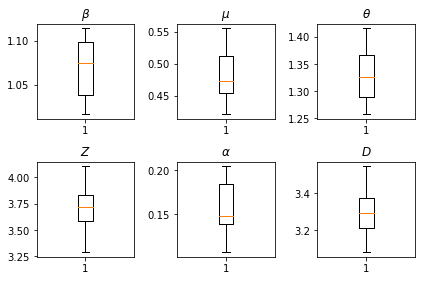
Hasil kesimpulan kami. Kami plot nilai kemungkinan maksimum untuk semua paramters global untuk menunjukkan variasi mereka di seluruh kami num_batches berjalan independen inferensi. Ini sesuai dengan Tabel S1 dalam bahan tambahan.
fig, axs = plt.subplots(2, 3)
axs[0, 0].boxplot(best_parameters.documented_infectious_tx_rate,
                  whis=(2.5,97.5), sym='')
axs[0, 0].set_title(r'$\beta$')

axs[0, 1].boxplot(best_parameters.undocumented_infectious_tx_relative_rate,
                  whis=(2.5,97.5), sym='')
axs[0, 1].set_title(r'$\mu$')

axs[0, 2].boxplot(best_parameters.intercity_underreporting_factor,
                  whis=(2.5,97.5), sym='')
axs[0, 2].set_title(r'$\theta$')

axs[1, 0].boxplot(best_parameters.average_latency_period,
                  whis=(2.5,97.5), sym='')
axs[1, 0].set_title(r'$Z$')

axs[1, 1].boxplot(best_parameters.fraction_of_documented_infections,
                  whis=(2.5,97.5), sym='')
axs[1, 1].set_title(r'$\alpha$')

axs[1, 2].boxplot(best_parameters.average_infection_duration,
                  whis=(2.5,97.5), sym='')
axs[1, 2].set_title(r'$D$')
plt.tight_layout()