
| | |  GitHub에서 소스 보기 GitHub에서 소스 보기 | |
에서 만든 비교의 오프 구축 MNIST의 튜토리얼이 튜토리얼의 최근 작업 탐구 황 등을. 다른 데이터 세트가 성능 비교에 미치는 영향을 보여줍니다. 이 작업에서 저자는 고전적인 기계 학습 모델이 양자 모델뿐만 아니라(또는 그 이상) 학습할 수 있는 방법과 시기를 이해하려고 합니다. 이 작업은 또한 신중하게 제작된 데이터 세트를 통해 클래식 및 양자 머신 러닝 모델 간의 경험적 성능 분리를 보여줍니다. 당신은:
- 축소된 차원의 Fashion-MNIST 데이터 세트를 준비합니다.
- 양자 회로를 사용하여 데이터 세트에 레이블을 다시 지정하고 PQK(Projected Quantum Kernel) 기능을 계산합니다.
- 레이블이 다시 지정된 데이터 세트에서 기존 신경망을 훈련시키고 PQK 기능에 액세스할 수 있는 모델과 성능을 비교합니다.
설정
pip install tensorflow==2.4.1 tensorflow-quantum
# Update package resources to account for version changes.
import importlib, pkg_resources
importlib.reload(pkg_resources)
import cirq
import sympy
import numpy as np
import tensorflow as tf
import tensorflow_quantum as tfq

# visualization tools
%matplotlib inline
import matplotlib.pyplot as plt
from cirq.contrib.svg import SVGCircuit
np.random.seed(1234)
1. 데이터 준비
양자 컴퓨터에서 실행할 패션 MNIST 데이터 세트를 준비하는 것으로 시작합니다.
1.1 패션-MNIST 다운로드
첫 번째 단계는 전통적인 fashion-mnist 데이터 세트를 얻는 것입니다. 이 작업은 사용하여 수행 할 수 있습니다 tf.keras.datasets 모듈을.
(x_train, y_train), (x_test, y_test) = tf.keras.datasets.fashion_mnist.load_data()

# Rescale the images from [0,255] to the [0.0,1.0] range.
x_train, x_test = x_train/255.0, x_test/255.0

print("Number of original training examples:", len(x_train))
print("Number of original test examples:", len(x_test))
Number of original training examples: 60000
Number of original test examples: 10000
데이터 세트를 필터링하여 티셔츠/상판 및 드레스만 유지하고 다른 클래스는 제거합니다. 동시에 변환 레이블에서, y , 부울합니다 : 0 참과 거짓을 3.
def filter_03(x, y):
    keep = (y == 0) | (y == 3)
    x, y = x[keep], y[keep]
    y = y == 0
    return x,y
x_train, y_train = filter_03(x_train, y_train)
x_test, y_test = filter_03(x_test, y_test)

print("Number of filtered training examples:", len(x_train))
print("Number of filtered test examples:", len(x_test))
Number of filtered training examples: 12000
Number of filtered test examples: 2000
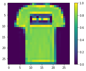
print(y_train[0])

plt.imshow(x_train[0, :, :])
plt.colorbar()
True
<matplotlib.colorbar.Colorbar at 0x7f6db42c3460>
1.2 이미지 축소
MNIST 예제와 마찬가지로 현재 양자 컴퓨터의 경계 내에 있도록 이러한 이미지를 축소해야 합니다. 이 시간은 그러나 당신은 치수 대신 줄이기 위해 PCA 변환을 사용합니다 tf.image.resize 작업을.
def truncate_x(x_train, x_test, n_components=10):
  """Perform PCA on image dataset keeping the top `n_components` components."""
  n_points_train = tf.gather(tf.shape(x_train), 0)
  n_points_test = tf.gather(tf.shape(x_test), 0)

  # Flatten to 1D
  x_train = tf.reshape(x_train, [n_points_train, -1])
  x_test = tf.reshape(x_test, [n_points_test, -1])

  # Normalize.
  feature_mean = tf.reduce_mean(x_train, axis=0)
  x_train_normalized = x_train - feature_mean
  x_test_normalized = x_test - feature_mean

  # Truncate.
  e_values, e_vectors = tf.linalg.eigh(
      tf.einsum('ji,jk->ik', x_train_normalized, x_train_normalized))
  return tf.einsum('ij,jk->ik', x_train_normalized, e_vectors[:,-n_components:]), \
    tf.einsum('ij,jk->ik', x_test_normalized, e_vectors[:, -n_components:])
DATASET_DIM = 10
x_train, x_test = truncate_x(x_train, x_test, n_components=DATASET_DIM)
print(f'New datapoint dimension:', len(x_train[0]))
New datapoint dimension: 10
마지막 단계는 데이터 세트의 크기를 훈련 데이터 포인트 1000개와 테스트 데이터 포인트 200개로 줄이는 것입니다.
N_TRAIN = 1000
N_TEST = 200
x_train, x_test = x_train[:N_TRAIN], x_test[:N_TEST]
y_train, y_test = y_train[:N_TRAIN], y_test[:N_TEST]
print("New number of training examples:", len(x_train))
print("New number of test examples:", len(x_test))
New number of training examples: 1000
New number of test examples: 200
2. PQK 기능의 레이블 재지정 및 계산
이제 양자 구성 요소를 통합하고 위에서 생성한 잘린 패션 MNIST 데이터 세트에 레이블을 다시 지정하여 "기울어진" 양자 데이터 세트를 준비합니다. 양자 방법과 기존 방법을 최대한 분리하기 위해 먼저 PQK 기능을 준비한 다음 해당 값에 따라 출력에 레이블을 다시 지정합니다.
2.1 양자 인코딩 및 PQK 기능
당신을 기반으로, 기능의 새로운 세트를 작성합니다 x_train , y_train , x_test 및 y_test 의 모든 큐 비트에 1 RDM으로 정의된다 :
\(V(x_{\text{train} } / n_{\text{trotter} }) ^ {n_{\text{trotter} } } U_{\text{1qb} } | 0 \rangle\)
어디 \(U_\text{1qb}\) 하나의 큐 비트 회전과의 벽입니다 \(V(\hat{\theta}) = e^{-i\sum_i \hat{\theta_i} (X_i X_{i+1} + Y_i Y_{i+1} + Z_i Z_{i+1})}\)
먼저 단일 큐비트 회전 벽을 생성할 수 있습니다.
def single_qubit_wall(qubits, rotations):
  """Prepare a single qubit X,Y,Z rotation wall on `qubits`."""
  wall_circuit = cirq.Circuit()
  for i, qubit in enumerate(qubits):
    for j, gate in enumerate([cirq.X, cirq.Y, cirq.Z]):
      wall_circuit.append(gate(qubit) ** rotations[i][j])

  return wall_circuit
회로를 살펴보면 이것이 작동하는지 빠르게 확인할 수 있습니다.
SVGCircuit(single_qubit_wall(
    cirq.GridQubit.rect(1,4), np.random.uniform(size=(4, 3))))

당신은 준비 할 수 다음으로 \(V(\hat{\theta})\) 의 도움으로 tfq.util.exponential 어떤 통근 exponentiate 수 cirq.PauliSum 객체 :
def v_theta(qubits):
  """Prepares a circuit that generates V(\theta)."""
  ref_paulis = [
      cirq.X(q0) * cirq.X(q1) + \
      cirq.Y(q0) * cirq.Y(q1) + \
      cirq.Z(q0) * cirq.Z(q1) for q0, q1 in zip(qubits, qubits[1:])
  ]
  exp_symbols = list(sympy.symbols('ref_0:'+str(len(ref_paulis))))
  return tfq.util.exponential(ref_paulis, exp_symbols), exp_symbols
이 회로는 보기로 확인하기가 조금 더 어려울 수 있지만 여전히 2큐비트 경우를 조사하여 무슨 일이 일어나고 있는지 확인할 수 있습니다.
test_circuit, test_symbols = v_theta(cirq.GridQubit.rect(1, 2))
print(f'Symbols found in circuit:{test_symbols}')
SVGCircuit(test_circuit)
Symbols found in circuit:[ref_0]

이제 전체 인코딩 회로를 결합하는 데 필요한 모든 구성 요소가 있습니다.
def prepare_pqk_circuits(qubits, classical_source, n_trotter=10):
  """Prepare the pqk feature circuits around a dataset."""
  n_qubits = len(qubits)
  n_points = len(classical_source)

  # Prepare random single qubit rotation wall.
  random_rots = np.random.uniform(-2, 2, size=(n_qubits, 3))
  initial_U = single_qubit_wall(qubits, random_rots)

  # Prepare parametrized V
  V_circuit, symbols = v_theta(qubits)
  exp_circuit = cirq.Circuit(V_circuit for t in range(n_trotter))

  # Convert to `tf.Tensor`
  initial_U_tensor = tfq.convert_to_tensor([initial_U])
  initial_U_splat = tf.tile(initial_U_tensor, [n_points])

  full_circuits = tfq.layers.AddCircuit()(
      initial_U_splat, append=exp_circuit)
  # Replace placeholders in circuits with values from `classical_source`.
  return tfq.resolve_parameters(
      full_circuits, tf.convert_to_tensor([str(x) for x in symbols]),
      tf.convert_to_tensor(classical_source*(n_qubits/3)/n_trotter))
일부 큐비트를 선택하고 데이터 인코딩 회로를 준비합니다.
qubits = cirq.GridQubit.rect(1, DATASET_DIM + 1)
q_x_train_circuits = prepare_pqk_circuits(qubits, x_train)
q_x_test_circuits = prepare_pqk_circuits(qubits, x_test)
다음에, PQK은 상기 데이터 세트 회로의 1 RDM에 기반 기능과 계산의 결과를 저장 rdm 하는 tf.Tensor 형상 [n_points, n_qubits, 3] . 의 항목 rdm[i][j][k] = \(\langle \psi_i | OP^k_j | \psi_i \rangle\) 여기서 i , 데이터 포인트 상에 인덱스 j 큐빗 이상의 인덱스 k 통해 인덱스 \(\lbrace \hat{X}, \hat{Y}, \hat{Z} \rbrace\) .
def get_pqk_features(qubits, data_batch):
  """Get PQK features based on above construction."""
  ops = [[cirq.X(q), cirq.Y(q), cirq.Z(q)] for q in qubits]
  ops_tensor = tf.expand_dims(tf.reshape(tfq.convert_to_tensor(ops), -1), 0)
  batch_dim = tf.gather(tf.shape(data_batch), 0)
  ops_splat = tf.tile(ops_tensor, [batch_dim, 1])
  exp_vals = tfq.layers.Expectation()(data_batch, operators=ops_splat)
  rdm = tf.reshape(exp_vals, [batch_dim, len(qubits), -1])
  return rdm
x_train_pqk = get_pqk_features(qubits, q_x_train_circuits)
x_test_pqk = get_pqk_features(qubits, q_x_test_circuits)
print('New PQK training dataset has shape:', x_train_pqk.shape)
print('New PQK testing dataset has shape:', x_test_pqk.shape)
New PQK training dataset has shape: (1000, 11, 3)
New PQK testing dataset has shape: (200, 11, 3)
2.2 PQK 기능을 기반으로 하는 재레이블링
이제 이러한 양자 생성 기능을 가지고 x_train_pqk 및 x_test_pqk , 그것은 다시 레이블 데이터 세트에 시간입니다. 양자하고 있습니다 고전 성능 사이의 최대 seperation에 달성하기 위해에있는 스펙트럼 정보를 기반으로 데이터 세트를 다시 레이블 x_train_pqk 및 x_test_pqk .
def compute_kernel_matrix(vecs, gamma):
  """Computes d[i][j] = e^ -gamma * (vecs[i] - vecs[j]) ** 2 """
  scaled_gamma = gamma / (
      tf.cast(tf.gather(tf.shape(vecs), 1), tf.float32) * tf.math.reduce_std(vecs))
  return scaled_gamma * tf.einsum('ijk->ij',(vecs[:,None,:] - vecs) ** 2)

def get_spectrum(datapoints, gamma=1.0):
  """Compute the eigenvalues and eigenvectors of the kernel of datapoints."""
  KC_qs = compute_kernel_matrix(datapoints, gamma)
  S, V = tf.linalg.eigh(KC_qs)
  S = tf.math.abs(S)
  return S, V
S_pqk, V_pqk = get_spectrum(
    tf.reshape(tf.concat([x_train_pqk, x_test_pqk], 0), [-1, len(qubits) * 3]))

S_original, V_original = get_spectrum(
    tf.cast(tf.concat([x_train, x_test], 0), tf.float32), gamma=0.005)

print('Eigenvectors of pqk kernel matrix:', V_pqk)
print('Eigenvectors of original kernel matrix:', V_original)
Eigenvectors of pqk kernel matrix: tf.Tensor(
[[-2.09569391e-02  1.05973557e-02  2.16634180e-02 ...  2.80352887e-02
   1.55521873e-02  2.82677952e-02]
 [-2.29303762e-02  4.66355234e-02  7.91163836e-03 ... -6.14174758e-04
  -7.07804322e-01  2.85902526e-02]
 [-1.77853629e-02 -3.00758495e-03 -2.55225878e-02 ... -2.40783971e-02
   2.11018627e-03  2.69009806e-02]
 ...
 [ 6.05797209e-02  1.32483775e-02  2.69536003e-02 ... -1.38843581e-02
   3.05043962e-02  3.85345481e-02]
 [ 6.33309558e-02 -3.04112374e-03  9.77444276e-03 ...  7.48321265e-02
   3.42793856e-03  3.67484428e-02]
 [ 5.86028099e-02  5.84433973e-03  2.64811981e-03 ...  2.82612257e-02
  -3.80136147e-02  3.29943895e-02]], shape=(1200, 1200), dtype=float32)
Eigenvectors of original kernel matrix: tf.Tensor(
[[ 0.03835681  0.0283473  -0.01169789 ...  0.02343717  0.0211248
   0.03206972]
 [-0.04018159  0.00888097 -0.01388255 ...  0.00582427  0.717551
   0.02881948]
 [-0.0166719   0.01350376 -0.03663862 ...  0.02467175 -0.00415936
   0.02195409]
 ...
 [-0.03015648 -0.01671632 -0.01603392 ...  0.00100583 -0.00261221
   0.02365689]
 [ 0.0039777  -0.04998879 -0.00528336 ...  0.01560401 -0.04330755
   0.02782002]
 [-0.01665728 -0.00818616 -0.0432341  ...  0.00088256  0.00927396
   0.01875088]], shape=(1200, 1200), dtype=float32)
이제 데이터 세트에 레이블을 다시 지정하는 데 필요한 모든 것이 준비되었습니다! 이제 데이터 세트에 레이블을 다시 지정할 때 성능 분리를 최대화하는 방법을 더 잘 이해하기 위해 순서도를 참조할 수 있습니다.
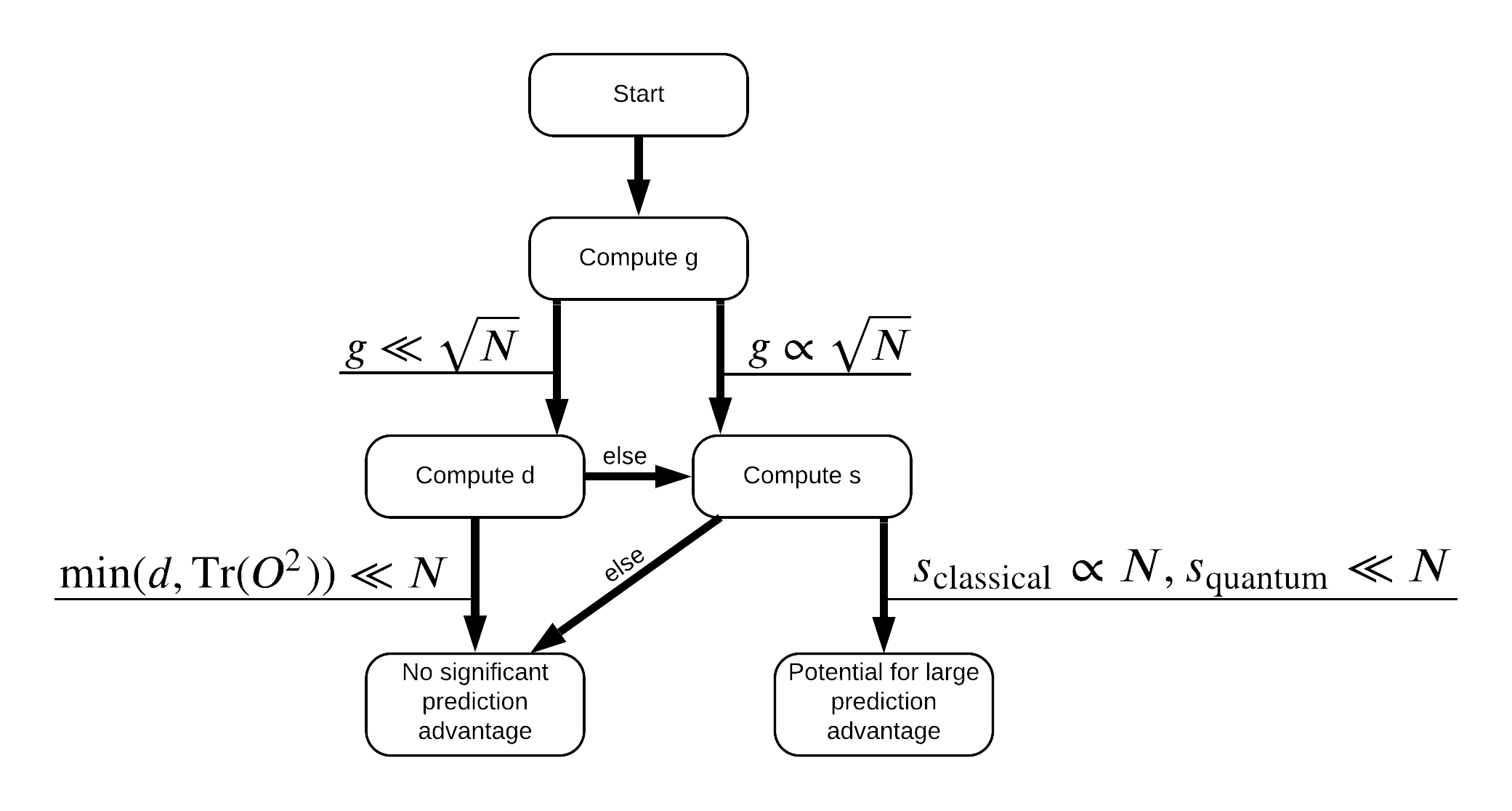
양자 클래식 모델 사이의 단락 지을 극대화하기 위해, 당신은 원본 데이터 셋 사이의 기하학적 차이를 극대화하려고 시도하고 PQK 커널 행렬 기능 \(g(K_1 || K_2) = \sqrt{ || \sqrt{K_2} K_1^{-1} \sqrt{K_2} || _\infty}\) 사용 S_pqk, V_pqk 및 S_original, V_original . 의 큰 값 \(g\) 보장하지만은 처음에는 양자의 경우에, 예측을 이용 향해 흐름도 아래에서 오른쪽으로 이동할 것이다.
def get_stilted_dataset(S, V, S_2, V_2, lambdav=1.1):
  """Prepare new labels that maximize geometric distance between kernels."""
  S_diag = tf.linalg.diag(S ** 0.5)
  S_2_diag = tf.linalg.diag(S_2 / (S_2 + lambdav) ** 2)
  scaling = S_diag @ tf.transpose(V) @ \
            V_2 @ S_2_diag @ tf.transpose(V_2) @ \
            V @ S_diag

  # Generate new lables using the largest eigenvector.
  _, vecs = tf.linalg.eig(scaling)
  new_labels = tf.math.real(
      tf.einsum('ij,j->i', tf.cast(V @ S_diag, tf.complex64), vecs[-1])).numpy()
  # Create new labels and add some small amount of noise.
  final_y = new_labels > np.median(new_labels)
  noisy_y = (final_y ^ (np.random.uniform(size=final_y.shape) > 0.95))
  return noisy_y
y_relabel = get_stilted_dataset(S_pqk, V_pqk, S_original, V_original)
y_train_new, y_test_new = y_relabel[:N_TRAIN], y_relabel[N_TRAIN:]
3. 모델 비교
데이터 세트를 준비했으므로 이제 모델 성능을 비교할 차례입니다. 당신은 두 개의 작은 피드 포워드 신경망을 만들고 그들이에서 발견되는 특징 PQK에 대한 액세스 권한을 부여 할 때 성능을 비교합니다 x_train_pqk .
3.1 PQK 강화 모델 생성
표준 사용 tf.keras 라이브러리 당신이 지금 만들 수있는 기능과 열차의 모델 x_train_pqk 및 y_train_new 데이터 포인트를 :
#docs_infra: no_execute
def create_pqk_model():
    model = tf.keras.Sequential()
    model.add(tf.keras.layers.Dense(32, activation='sigmoid', input_shape=[len(qubits) * 3,]))
    model.add(tf.keras.layers.Dense(16, activation='sigmoid'))
    model.add(tf.keras.layers.Dense(1))
    return model

pqk_model = create_pqk_model()
pqk_model.compile(loss=tf.keras.losses.BinaryCrossentropy(from_logits=True),
              optimizer=tf.keras.optimizers.Adam(learning_rate=0.003),
              metrics=['accuracy'])

pqk_model.summary()
Model: "sequential"
_________________________________________________________________
Layer (type)                 Output Shape              Param #
=================================================================
dense (Dense)                (None, 32)                1088
_________________________________________________________________
dense_1 (Dense)              (None, 16)                528
_________________________________________________________________
dense_2 (Dense)              (None, 1)                 17
=================================================================
Total params: 1,633
Trainable params: 1,633
Non-trainable params: 0
_________________________________________________________________
#docs_infra: no_execute
pqk_history = pqk_model.fit(tf.reshape(x_train_pqk, [N_TRAIN, -1]),
          y_train_new,
          batch_size=32,
          epochs=1000,
          verbose=0,
          validation_data=(tf.reshape(x_test_pqk, [N_TEST, -1]), y_test_new))
3.2 클래식 모델 만들기
위의 코드와 유사하게 이제 stilted 데이터세트의 PQK 기능에 액세스할 수 없는 클래식 모델을 만들 수도 있습니다. 이 모델은 사용 훈련을 할 수 x_train 및 y_label_new .
#docs_infra: no_execute
def create_fair_classical_model():
    model = tf.keras.Sequential()
    model.add(tf.keras.layers.Dense(32, activation='sigmoid', input_shape=[DATASET_DIM,]))
    model.add(tf.keras.layers.Dense(16, activation='sigmoid'))
    model.add(tf.keras.layers.Dense(1))
    return model

model = create_fair_classical_model()
model.compile(loss=tf.keras.losses.BinaryCrossentropy(from_logits=True),
              optimizer=tf.keras.optimizers.Adam(learning_rate=0.03),
              metrics=['accuracy'])

model.summary()
Model: "sequential_1"
_________________________________________________________________
Layer (type)                 Output Shape              Param #
=================================================================
dense_3 (Dense)              (None, 32)                352
_________________________________________________________________
dense_4 (Dense)              (None, 16)                528
_________________________________________________________________
dense_5 (Dense)              (None, 1)                 17
=================================================================
Total params: 897
Trainable params: 897
Non-trainable params: 0
_________________________________________________________________
#docs_infra: no_execute
classical_history = model.fit(x_train,
          y_train_new,
          batch_size=32,
          epochs=1000,
          verbose=0,
          validation_data=(x_test, y_test_new))
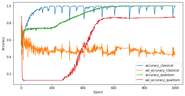
3.3 성능 비교
이제 두 모델을 훈련했으므로 둘 사이의 유효성 검사 데이터에서 성능 격차를 빠르게 플롯할 수 있습니다. 일반적으로 두 모델 모두 훈련 데이터에서 > 0.9 정확도를 달성합니다. 그러나 검증 데이터에서 PQK 기능에서 발견된 정보만이 모델을 보이지 않는 인스턴스에 잘 일반화할 수 있도록 하기에 충분하다는 것이 분명해졌습니다.
#docs_infra: no_execute
plt.figure(figsize=(10,5))
plt.plot(classical_history.history['accuracy'], label='accuracy_classical')
plt.plot(classical_history.history['val_accuracy'], label='val_accuracy_classical')
plt.plot(pqk_history.history['accuracy'], label='accuracy_quantum')
plt.plot(pqk_history.history['val_accuracy'], label='val_accuracy_quantum')
plt.xlabel('Epoch')
plt.ylabel('Accuracy')
plt.legend()
<matplotlib.legend.Legend at 0x7f6d846ecee0>
4. 중요한 결론
이과에서 그릴 수있는 몇 가지 중요한 결론이 있습니다 MNIST의 실험 :
오늘날의 양자 모델이 고전 데이터에서 고전 모델 성능을 능가할 가능성은 거의 없습니다. 특히 백만 개 이상의 데이터 포인트를 가질 수 있는 오늘날의 기존 데이터 세트에서는 더욱 그렇습니다.
데이터가 고전적으로 시뮬레이션하기 어려운 양자 회로에서 나올 수 있다고 해서 반드시 고전 모델에서 데이터를 학습하기 어렵게 만드는 것은 아닙니다.
사용된 모델 아키텍처나 훈련 알고리즘에 관계없이 양자 모델이 배우기 쉽고 고전적 모델이 배우기 어려운 데이터 세트(궁극적으로는 본질적으로 양자)는 존재합니다.