
| | |  Xem nguồn trên GitHub Xem nguồn trên GitHub | |
Xây dựng tắt của sự so sánh được thực hiện trong MNIST hướng dẫn, hướng dẫn này khám phá những công việc gần đây của Huang et al. điều đó cho thấy các bộ dữ liệu khác nhau ảnh hưởng như thế nào đến việc so sánh hiệu suất. Trong tác phẩm, các tác giả tìm cách hiểu làm thế nào và khi nào các mô hình học máy cổ điển có thể học tốt như (hoặc tốt hơn) các mô hình lượng tử. Công trình cũng giới thiệu sự phân tách hiệu suất thực nghiệm giữa mô hình học máy lượng tử và cổ điển thông qua một tập dữ liệu được xây dựng cẩn thận. Bạn sẽ:
- Chuẩn bị tập dữ liệu Fashion-MNIST thứ nguyên giảm.
- Sử dụng mạch lượng tử để gắn nhãn lại tập dữ liệu và tính toán các đặc điểm của Hạt nhân lượng tử dự kiến (PQK).
- Đào tạo mạng nơ-ron cổ điển trên tập dữ liệu được gắn nhãn lại và so sánh hiệu suất với mô hình có quyền truy cập vào các tính năng PQK.
Thành lập
pip install tensorflow==2.4.1 tensorflow-quantum
# Update package resources to account for version changes.
import importlib, pkg_resources
importlib.reload(pkg_resources)
import cirq
import sympy
import numpy as np
import tensorflow as tf
import tensorflow_quantum as tfq

# visualization tools
%matplotlib inline
import matplotlib.pyplot as plt
from cirq.contrib.svg import SVGCircuit
np.random.seed(1234)
1. Chuẩn bị dữ liệu
Bạn sẽ bắt đầu bằng cách chuẩn bị bộ dữ liệu thời trang-MNIST để chạy trên máy tính lượng tử.
1.1 Tải xuống fashion-MNIST
Bước đầu tiên là lấy bộ dữ liệu thời trang truyền thống. Điều này có thể được thực hiện bằng cách sử dụng tf.keras.datasets module.
(x_train, y_train), (x_test, y_test) = tf.keras.datasets.fashion_mnist.load_data()

# Rescale the images from [0,255] to the [0.0,1.0] range.
x_train, x_test = x_train/255.0, x_test/255.0

print("Number of original training examples:", len(x_train))
print("Number of original test examples:", len(x_test))
Number of original training examples: 60000
Number of original test examples: 10000
Lọc tập dữ liệu để chỉ giữ lại áo phông / áo sơ mi và váy, loại bỏ các lớp khác. Tại cùng một thời gian chuyển đổi nhãn, y , để boolean: True cho 0 và False cho 3.
def filter_03(x, y):
    keep = (y == 0) | (y == 3)
    x, y = x[keep], y[keep]
    y = y == 0
    return x,y
x_train, y_train = filter_03(x_train, y_train)
x_test, y_test = filter_03(x_test, y_test)

print("Number of filtered training examples:", len(x_train))
print("Number of filtered test examples:", len(x_test))
Number of filtered training examples: 12000
Number of filtered test examples: 2000
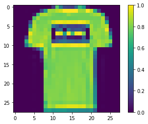
print(y_train[0])

plt.imshow(x_train[0, :, :])
plt.colorbar()
True
<matplotlib.colorbar.Colorbar at 0x7f6db42c3460>
1.2 Giảm tỷ lệ hình ảnh
Cũng giống như ví dụ MNIST, bạn sẽ cần giảm tỷ lệ những hình ảnh này để nằm trong ranh giới của các máy tính lượng tử hiện tại. Tuy nhiên lần này bạn sẽ sử dụng một chuyển đổi PCA để giảm kích thước thay vì một tf.image.resize hoạt động.
def truncate_x(x_train, x_test, n_components=10):
  """Perform PCA on image dataset keeping the top `n_components` components."""
  n_points_train = tf.gather(tf.shape(x_train), 0)
  n_points_test = tf.gather(tf.shape(x_test), 0)

  # Flatten to 1D
  x_train = tf.reshape(x_train, [n_points_train, -1])
  x_test = tf.reshape(x_test, [n_points_test, -1])

  # Normalize.
  feature_mean = tf.reduce_mean(x_train, axis=0)
  x_train_normalized = x_train - feature_mean
  x_test_normalized = x_test - feature_mean

  # Truncate.
  e_values, e_vectors = tf.linalg.eigh(
      tf.einsum('ji,jk->ik', x_train_normalized, x_train_normalized))
  return tf.einsum('ij,jk->ik', x_train_normalized, e_vectors[:,-n_components:]), \
    tf.einsum('ij,jk->ik', x_test_normalized, e_vectors[:, -n_components:])
DATASET_DIM = 10
x_train, x_test = truncate_x(x_train, x_test, n_components=DATASET_DIM)
print(f'New datapoint dimension:', len(x_train[0]))
New datapoint dimension: 10
Bước cuối cùng là giảm kích thước của tập dữ liệu xuống chỉ còn 1000 điểm dữ liệu đào tạo và 200 điểm dữ liệu thử nghiệm.
N_TRAIN = 1000
N_TEST = 200
x_train, x_test = x_train[:N_TRAIN], x_test[:N_TEST]
y_train, y_test = y_train[:N_TRAIN], y_test[:N_TEST]
print("New number of training examples:", len(x_train))
print("New number of test examples:", len(x_test))
New number of training examples: 1000
New number of test examples: 200
2. Tái gắn nhãn và tính toán các tính năng PQK
Bây giờ bạn sẽ chuẩn bị một tập dữ liệu lượng tử "cố định" bằng cách kết hợp các thành phần lượng tử và dán nhãn lại cho tập dữ liệu MNIST thời trang đã được cắt ngắn mà bạn đã tạo ở trên. Để có được sự tách biệt nhất giữa phương pháp lượng tử và phương pháp cổ điển, trước tiên bạn sẽ chuẩn bị các tính năng PQK và sau đó gắn nhãn lại các kết quả đầu ra dựa trên giá trị của chúng.
2.1 Mã hóa lượng tử và các tính năng PQK
Bạn sẽ tạo ra một tập hợp mới các tính năng, dựa trên x_train , y_train , x_test và y_test được định nghĩa là 1-RDM trên tất cả các qubit của:
\(V(x_{\text{train} } / n_{\text{trotter} }) ^ {n_{\text{trotter} } } U_{\text{1qb} } | 0 \rangle\)
Nơi \(U_\text{1qb}\) là một bức tường quay qubit đơn và \(V(\hat{\theta}) = e^{-i\sum_i \hat{\theta_i} (X_i X_{i+1} + Y_i Y_{i+1} + Z_i Z_{i+1})}\)
Đầu tiên, bạn có thể tạo bức tường của các phép quay qubit đơn lẻ:
def single_qubit_wall(qubits, rotations):
  """Prepare a single qubit X,Y,Z rotation wall on `qubits`."""
  wall_circuit = cirq.Circuit()
  for i, qubit in enumerate(qubits):
    for j, gate in enumerate([cirq.X, cirq.Y, cirq.Z]):
      wall_circuit.append(gate(qubit) ** rotations[i][j])

  return wall_circuit
Bạn có thể nhanh chóng xác minh điều này hoạt động bằng cách xem mạch:
SVGCircuit(single_qubit_wall(
    cirq.GridQubit.rect(1,4), np.random.uniform(size=(4, 3))))

Tiếp theo, bạn có thể chuẩn bị \(V(\hat{\theta})\) với sự giúp đỡ của tfq.util.exponential có thể exponentiate bất kỳ đi lại cirq.PauliSum các đối tượng:
def v_theta(qubits):
  """Prepares a circuit that generates V(\theta)."""
  ref_paulis = [
      cirq.X(q0) * cirq.X(q1) + \
      cirq.Y(q0) * cirq.Y(q1) + \
      cirq.Z(q0) * cirq.Z(q1) for q0, q1 in zip(qubits, qubits[1:])
  ]
  exp_symbols = list(sympy.symbols('ref_0:'+str(len(ref_paulis))))
  return tfq.util.exponential(ref_paulis, exp_symbols), exp_symbols
Mạch này có thể khó xác minh hơn một chút bằng cách xem xét, nhưng bạn vẫn có thể kiểm tra trường hợp hai qubit để xem điều gì đang xảy ra:
test_circuit, test_symbols = v_theta(cirq.GridQubit.rect(1, 2))
print(f'Symbols found in circuit:{test_symbols}')
SVGCircuit(test_circuit)
Symbols found in circuit:[ref_0]

Bây giờ bạn có tất cả các khối xây dựng mà bạn cần để ghép các mạch mã hóa đầy đủ của mình lại với nhau:
def prepare_pqk_circuits(qubits, classical_source, n_trotter=10):
  """Prepare the pqk feature circuits around a dataset."""
  n_qubits = len(qubits)
  n_points = len(classical_source)

  # Prepare random single qubit rotation wall.
  random_rots = np.random.uniform(-2, 2, size=(n_qubits, 3))
  initial_U = single_qubit_wall(qubits, random_rots)

  # Prepare parametrized V
  V_circuit, symbols = v_theta(qubits)
  exp_circuit = cirq.Circuit(V_circuit for t in range(n_trotter))

  # Convert to `tf.Tensor`
  initial_U_tensor = tfq.convert_to_tensor([initial_U])
  initial_U_splat = tf.tile(initial_U_tensor, [n_points])

  full_circuits = tfq.layers.AddCircuit()(
      initial_U_splat, append=exp_circuit)
  # Replace placeholders in circuits with values from `classical_source`.
  return tfq.resolve_parameters(
      full_circuits, tf.convert_to_tensor([str(x) for x in symbols]),
      tf.convert_to_tensor(classical_source*(n_qubits/3)/n_trotter))
Chọn một số qubit và chuẩn bị mạch mã hóa dữ liệu:
qubits = cirq.GridQubit.rect(1, DATASET_DIM + 1)
q_x_train_circuits = prepare_pqk_circuits(qubits, x_train)
q_x_test_circuits = prepare_pqk_circuits(qubits, x_test)
Tiếp theo, tính toán PQK các tính năng dựa trên 1-RDM của các mạch số liệu trên và lưu trữ các kết quả trong rdm , một tf.Tensor với hình dạng [n_points, n_qubits, 3] . Các mục trong rdm[i][j][k] = \(\langle \psi_i | OP^k_j | \psi_i \rangle\) nơi i chỉ trên datapoints, j chỉ số trên qubit và k chỉ số trên \(\lbrace \hat{X}, \hat{Y}, \hat{Z} \rbrace\) .
def get_pqk_features(qubits, data_batch):
  """Get PQK features based on above construction."""
  ops = [[cirq.X(q), cirq.Y(q), cirq.Z(q)] for q in qubits]
  ops_tensor = tf.expand_dims(tf.reshape(tfq.convert_to_tensor(ops), -1), 0)
  batch_dim = tf.gather(tf.shape(data_batch), 0)
  ops_splat = tf.tile(ops_tensor, [batch_dim, 1])
  exp_vals = tfq.layers.Expectation()(data_batch, operators=ops_splat)
  rdm = tf.reshape(exp_vals, [batch_dim, len(qubits), -1])
  return rdm
x_train_pqk = get_pqk_features(qubits, q_x_train_circuits)
x_test_pqk = get_pqk_features(qubits, q_x_test_circuits)
print('New PQK training dataset has shape:', x_train_pqk.shape)
print('New PQK testing dataset has shape:', x_test_pqk.shape)
New PQK training dataset has shape: (1000, 11, 3)
New PQK testing dataset has shape: (200, 11, 3)
2.2 Dán nhãn lại dựa trên các tính năng PQK
Bây giờ bạn có các tính năng lượng tử tạo ra trong x_train_pqk và x_test_pqk , đó là thời gian để tái nhãn dataset. Để đạt được tách tối đa giữa lượng tử và hiệu suất cổ điển, bạn có thể tái nhãn dữ liệu dựa trên các thông tin tìm thấy trong quang phổ x_train_pqk và x_test_pqk .
def compute_kernel_matrix(vecs, gamma):
  """Computes d[i][j] = e^ -gamma * (vecs[i] - vecs[j]) ** 2 """
  scaled_gamma = gamma / (
      tf.cast(tf.gather(tf.shape(vecs), 1), tf.float32) * tf.math.reduce_std(vecs))
  return scaled_gamma * tf.einsum('ijk->ij',(vecs[:,None,:] - vecs) ** 2)

def get_spectrum(datapoints, gamma=1.0):
  """Compute the eigenvalues and eigenvectors of the kernel of datapoints."""
  KC_qs = compute_kernel_matrix(datapoints, gamma)
  S, V = tf.linalg.eigh(KC_qs)
  S = tf.math.abs(S)
  return S, V
S_pqk, V_pqk = get_spectrum(
    tf.reshape(tf.concat([x_train_pqk, x_test_pqk], 0), [-1, len(qubits) * 3]))

S_original, V_original = get_spectrum(
    tf.cast(tf.concat([x_train, x_test], 0), tf.float32), gamma=0.005)

print('Eigenvectors of pqk kernel matrix:', V_pqk)
print('Eigenvectors of original kernel matrix:', V_original)
Eigenvectors of pqk kernel matrix: tf.Tensor(
[[-2.09569391e-02  1.05973557e-02  2.16634180e-02 ...  2.80352887e-02
   1.55521873e-02  2.82677952e-02]
 [-2.29303762e-02  4.66355234e-02  7.91163836e-03 ... -6.14174758e-04
  -7.07804322e-01  2.85902526e-02]
 [-1.77853629e-02 -3.00758495e-03 -2.55225878e-02 ... -2.40783971e-02
   2.11018627e-03  2.69009806e-02]
 ...
 [ 6.05797209e-02  1.32483775e-02  2.69536003e-02 ... -1.38843581e-02
   3.05043962e-02  3.85345481e-02]
 [ 6.33309558e-02 -3.04112374e-03  9.77444276e-03 ...  7.48321265e-02
   3.42793856e-03  3.67484428e-02]
 [ 5.86028099e-02  5.84433973e-03  2.64811981e-03 ...  2.82612257e-02
  -3.80136147e-02  3.29943895e-02]], shape=(1200, 1200), dtype=float32)
Eigenvectors of original kernel matrix: tf.Tensor(
[[ 0.03835681  0.0283473  -0.01169789 ...  0.02343717  0.0211248
   0.03206972]
 [-0.04018159  0.00888097 -0.01388255 ...  0.00582427  0.717551
   0.02881948]
 [-0.0166719   0.01350376 -0.03663862 ...  0.02467175 -0.00415936
   0.02195409]
 ...
 [-0.03015648 -0.01671632 -0.01603392 ...  0.00100583 -0.00261221
   0.02365689]
 [ 0.0039777  -0.04998879 -0.00528336 ...  0.01560401 -0.04330755
   0.02782002]
 [-0.01665728 -0.00818616 -0.0432341  ...  0.00088256  0.00927396
   0.01875088]], shape=(1200, 1200), dtype=float32)
Bây giờ bạn có mọi thứ bạn cần để gắn nhãn lại tập dữ liệu! Bây giờ, bạn có thể tham khảo lưu đồ để hiểu rõ hơn về cách tối đa hóa phân tách hiệu suất khi gắn nhãn lại tập dữ liệu:
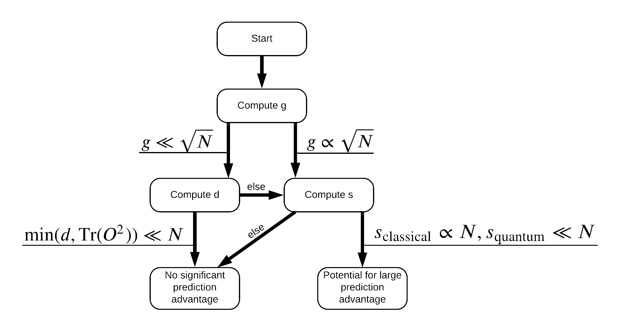
Để tối đa hóa sự chia tách giữa lượng tử và mô hình cổ điển, bạn sẽ cố gắng tối đa hóa sự khác biệt hình học giữa các bộ dữ liệu gốc và PQK tính năng hạt nhân ma trận \(g(K_1 || K_2) = \sqrt{ || \sqrt{K_2} K_1^{-1} \sqrt{K_2} || _\infty}\) sử dụng S_pqk, V_pqk và S_original, V_original . Một giá trị lớn \(g\) đảm bảo rằng bạn ban đầu chuyển sang bên phải trong sơ đồ xuống hướng tới một lợi thế dự đoán trong trường hợp lượng tử.
def get_stilted_dataset(S, V, S_2, V_2, lambdav=1.1):
  """Prepare new labels that maximize geometric distance between kernels."""
  S_diag = tf.linalg.diag(S ** 0.5)
  S_2_diag = tf.linalg.diag(S_2 / (S_2 + lambdav) ** 2)
  scaling = S_diag @ tf.transpose(V) @ \
            V_2 @ S_2_diag @ tf.transpose(V_2) @ \
            V @ S_diag

  # Generate new lables using the largest eigenvector.
  _, vecs = tf.linalg.eig(scaling)
  new_labels = tf.math.real(
      tf.einsum('ij,j->i', tf.cast(V @ S_diag, tf.complex64), vecs[-1])).numpy()
  # Create new labels and add some small amount of noise.
  final_y = new_labels > np.median(new_labels)
  noisy_y = (final_y ^ (np.random.uniform(size=final_y.shape) > 0.95))
  return noisy_y
y_relabel = get_stilted_dataset(S_pqk, V_pqk, S_original, V_original)
y_train_new, y_test_new = y_relabel[:N_TRAIN], y_relabel[N_TRAIN:]
3. So sánh các mô hình
Bây giờ bạn đã chuẩn bị tập dữ liệu của mình, đã đến lúc so sánh hiệu suất của mô hình. Bạn sẽ tạo ra hai mạng nơ-ron feedforward nhỏ và so sánh hiệu suất khi họ được tiếp cận với PQK tính năng tìm thấy trong x_train_pqk .
3.1 Tạo mô hình nâng cao PQK
Sử dụng tiêu chuẩn tf.keras tính năng thư viện bây giờ bạn có thể tạo và một con tàu mô hình trên x_train_pqk và y_train_new datapoints:
#docs_infra: no_execute
def create_pqk_model():
    model = tf.keras.Sequential()
    model.add(tf.keras.layers.Dense(32, activation='sigmoid', input_shape=[len(qubits) * 3,]))
    model.add(tf.keras.layers.Dense(16, activation='sigmoid'))
    model.add(tf.keras.layers.Dense(1))
    return model

pqk_model = create_pqk_model()
pqk_model.compile(loss=tf.keras.losses.BinaryCrossentropy(from_logits=True),
              optimizer=tf.keras.optimizers.Adam(learning_rate=0.003),
              metrics=['accuracy'])

pqk_model.summary()
Model: "sequential"
_________________________________________________________________
Layer (type)                 Output Shape              Param #
=================================================================
dense (Dense)                (None, 32)                1088
_________________________________________________________________
dense_1 (Dense)              (None, 16)                528
_________________________________________________________________
dense_2 (Dense)              (None, 1)                 17
=================================================================
Total params: 1,633
Trainable params: 1,633
Non-trainable params: 0
_________________________________________________________________
#docs_infra: no_execute
pqk_history = pqk_model.fit(tf.reshape(x_train_pqk, [N_TRAIN, -1]),
          y_train_new,
          batch_size=32,
          epochs=1000,
          verbose=0,
          validation_data=(tf.reshape(x_test_pqk, [N_TEST, -1]), y_test_new))
3.2 Tạo một mô hình cổ điển
Tương tự như đoạn mã ở trên, bây giờ bạn cũng có thể tạo một mô hình cổ điển không có quyền truy cập vào các tính năng PQK trong tập dữ liệu cố định của mình. Mô hình này có thể được huấn luyện sử dụng x_train và y_label_new .
#docs_infra: no_execute
def create_fair_classical_model():
    model = tf.keras.Sequential()
    model.add(tf.keras.layers.Dense(32, activation='sigmoid', input_shape=[DATASET_DIM,]))
    model.add(tf.keras.layers.Dense(16, activation='sigmoid'))
    model.add(tf.keras.layers.Dense(1))
    return model

model = create_fair_classical_model()
model.compile(loss=tf.keras.losses.BinaryCrossentropy(from_logits=True),
              optimizer=tf.keras.optimizers.Adam(learning_rate=0.03),
              metrics=['accuracy'])

model.summary()
Model: "sequential_1"
_________________________________________________________________
Layer (type)                 Output Shape              Param #
=================================================================
dense_3 (Dense)              (None, 32)                352
_________________________________________________________________
dense_4 (Dense)              (None, 16)                528
_________________________________________________________________
dense_5 (Dense)              (None, 1)                 17
=================================================================
Total params: 897
Trainable params: 897
Non-trainable params: 0
_________________________________________________________________
#docs_infra: no_execute
classical_history = model.fit(x_train,
          y_train_new,
          batch_size=32,
          epochs=1000,
          verbose=0,
          validation_data=(x_test, y_test_new))
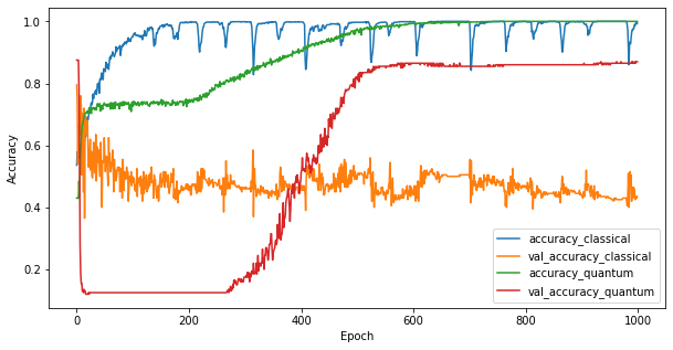
3.3 So sánh hiệu suất
Bây giờ bạn đã đào tạo hai mô hình, bạn có thể nhanh chóng vẽ biểu đồ khoảng cách hiệu suất trong dữ liệu xác thực giữa hai mô hình. Thông thường, cả hai mô hình sẽ đạt được độ chính xác> 0,9 trên dữ liệu đào tạo. Tuy nhiên, trên dữ liệu xác thực, rõ ràng là chỉ thông tin được tìm thấy trong các tính năng PQK là đủ để làm cho mô hình tổng quát hóa tốt cho các trường hợp không nhìn thấy.
#docs_infra: no_execute
plt.figure(figsize=(10,5))
plt.plot(classical_history.history['accuracy'], label='accuracy_classical')
plt.plot(classical_history.history['val_accuracy'], label='val_accuracy_classical')
plt.plot(pqk_history.history['accuracy'], label='accuracy_quantum')
plt.plot(pqk_history.history['val_accuracy'], label='val_accuracy_quantum')
plt.xlabel('Epoch')
plt.ylabel('Accuracy')
plt.legend()
<matplotlib.legend.Legend at 0x7f6d846ecee0>
4. Kết luận quan trọng
Có một số kết luận quan trọng, bạn có thể rút ra từ này và MNIST thí nghiệm:
Rất ít khả năng các mô hình lượng tử ngày nay sẽ đánh bại hiệu suất mô hình cổ điển trên dữ liệu cổ điển. Đặc biệt là trên các bộ dữ liệu cổ điển ngày nay có thể có tới một triệu điểm dữ liệu.
Chỉ vì dữ liệu có thể đến từ một mạch lượng tử khó mô phỏng theo kiểu cổ điển, không nhất thiết phải làm cho dữ liệu khó học đối với một mô hình cổ điển.
Các tập dữ liệu (cuối cùng về bản chất là lượng tử) dễ dàng cho các mô hình lượng tử học và các mô hình cổ điển khó học vẫn tồn tại, bất kể kiến trúc mô hình hoặc các thuật toán đào tạo được sử dụng.