
| | |  GitHub에서 소스 보기 GitHub에서 소스 보기 | |
TensorFlow Quantum은 양자 프리미티브를 TensorFlow 생태계로 가져옵니다. 이제 양자 연구자는 TensorFlow의 도구를 활용할 수 있습니다. 이 자습서에서는 TensorBoard 를 양자 컴퓨팅 연구에 통합하는 방법을 자세히 살펴봅니다. TensorFlow의 DCGAN 튜토리얼 을 사용하면 Niu 등이 수행한 것과 유사한 작업 실험 및 시각화를 빠르게 구축할 수 있습니다. . 일반적으로 다음을 수행합니다.
- GAN을 훈련하여 양자 회로에서 온 것처럼 보이는 샘플을 생성합니다.
- 교육 진행 상황과 시간 경과에 따른 분포 변화를 시각화합니다.
- 컴퓨팅 그래프를 탐색하여 실험을 벤치마킹합니다.
pip install tensorflow==2.7.0 tensorflow-quantum tensorboard_plugin_profile==2.4.0
# Update package resources to account for version changes.
import importlib, pkg_resources
importlib.reload(pkg_resources)
<module 'pkg_resources' from '/tmpfs/src/tf_docs_env/lib/python3.7/site-packages/pkg_resources/__init__.py'>
#docs_infra: no_execute
%load_ext tensorboard
import datetime
import time
import cirq
import tensorflow as tf
import tensorflow_quantum as tfq
from tensorflow.keras import layers

# visualization tools
%matplotlib inline
import matplotlib.pyplot as plt
from cirq.contrib.svg import SVGCircuit
2022-02-04 12:46:52.770534: E tensorflow/stream_executor/cuda/cuda_driver.cc:271] failed call to cuInit: CUDA_ERROR_NO_DEVICE: no CUDA-capable device is detected
1. 데이터 생성
몇 가지 데이터를 수집하여 시작하십시오. TensorFlow Quantum을 사용하여 나머지 실험의 기본 데이터 소스가 될 일부 비트열 샘플을 빠르게 생성할 수 있습니다. Niu et al. 대폭 감소된 깊이로 임의의 회로에서 샘플링을 에뮬레이트하는 것이 얼마나 쉬운지 탐색할 것입니다. 먼저 몇 가지 도우미를 정의합니다.
def generate_circuit(qubits):
    """Generate a random circuit on qubits."""
    random_circuit = cirq.generate_boixo_2018_supremacy_circuits_v2(
        qubits, cz_depth=2, seed=1234)
    return random_circuit

def generate_data(circuit, n_samples):
    """Draw n_samples samples from circuit into a tf.Tensor."""
    return tf.squeeze(tfq.layers.Sample()(circuit, repetitions=n_samples).to_tensor())
이제 회로와 일부 샘플 데이터를 검사할 수 있습니다.
qubits = cirq.GridQubit.rect(1, 5)
random_circuit_m = generate_circuit(qubits) + cirq.measure_each(*qubits)
SVGCircuit(random_circuit_m)
findfont: Font family ['Arial'] not found. Falling back to DejaVu Sans.

samples = cirq.sample(random_circuit_m, repetitions=10)
print('10 Random bitstrings from this circuit:')
print(samples)
10 Random bitstrings from this circuit:
(0, 0)=1000001000
(0, 1)=0000001010
(0, 2)=1010000100
(0, 3)=0010000110
(0, 4)=0110110010
다음을 사용하여 TensorFlow Quantum에서 동일한 작업을 수행할 수 있습니다.
generate_data(random_circuit_m, 10)
<tf.Tensor: shape=(10, 5), dtype=int8, numpy=
array([[0, 0, 0, 0, 0],
       [0, 0, 0, 0, 0],
       [0, 0, 1, 0, 0],
       [0, 1, 0, 0, 0],
       [0, 1, 0, 0, 0],
       [0, 1, 1, 0, 0],
       [1, 0, 0, 0, 0],
       [1, 0, 0, 1, 0],
       [1, 1, 1, 0, 0],
       [1, 1, 1, 0, 0]], dtype=int8)>
이제 다음을 사용하여 교육 데이터를 빠르게 생성할 수 있습니다.
N_SAMPLES = 60000
N_QUBITS = 10
QUBITS = cirq.GridQubit.rect(1, N_QUBITS)
REFERENCE_CIRCUIT = generate_circuit(QUBITS)
all_data = generate_data(REFERENCE_CIRCUIT, N_SAMPLES)
all_data
<tf.Tensor: shape=(60000, 10), dtype=int8, numpy=
array([[0, 0, 0, ..., 0, 0, 0],
       [0, 0, 0, ..., 0, 0, 0],
       [0, 0, 0, ..., 0, 0, 0],
       ...,
       [1, 1, 1, ..., 1, 1, 1],
       [1, 1, 1, ..., 1, 1, 1],
       [1, 1, 1, ..., 1, 1, 1]], dtype=int8)>
훈련이 진행됨에 따라 시각화할 몇 가지 도우미 함수를 정의하는 것이 유용할 것입니다. 사용할 두 가지 흥미로운 양은 다음과 같습니다.
- 분포의 히스토그램을 생성할 수 있도록 샘플의 정수 값.
- 샘플 집합의 선형 XEB 충실도 추정값으로 샘플이 얼마나 "진정한 양자 랜덤"인지에 대한 표시를 제공합니다.
@tf.function
def bits_to_ints(bits):
    """Convert tensor of bitstrings to tensor of ints."""
    sigs = tf.constant([1 << i for i in range(N_QUBITS)], dtype=tf.int32)
    rounded_bits = tf.clip_by_value(tf.math.round(
        tf.cast(bits, dtype=tf.dtypes.float32)), clip_value_min=0, clip_value_max=1)
    return tf.einsum('jk,k->j', tf.cast(rounded_bits, dtype=tf.dtypes.int32), sigs)

@tf.function
def xeb_fid(bits):
    """Compute linear XEB fidelity of bitstrings."""
    final_probs = tf.squeeze(
        tf.abs(tfq.layers.State()(REFERENCE_CIRCUIT).to_tensor()) ** 2)
    nums = bits_to_ints(bits)
    return (2 ** N_QUBITS) * tf.reduce_mean(tf.gather(final_probs, nums)) - 1.0
여기에서 XEB를 사용하여 배포 및 온전성 검사를 시각화할 수 있습니다.
plt.hist(bits_to_ints(all_data).numpy(), 50)
plt.show()
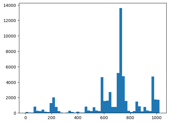
xeb_fid(all_data)
<tf.Tensor: shape=(), dtype=float32, numpy=-0.0015467405>
2. 모델 구축
여기에서 양자 사례에 대한 DCGAN 자습서 의 관련 구성 요소를 사용할 수 있습니다. MNIST 숫자를 생성하는 대신 새 GAN을 사용하여 길이가 N_QUBITS 비트열 샘플을 생성합니다.
LATENT_DIM = 100
def make_generator_model():
    """Construct generator model."""
    model = tf.keras.Sequential()
    model.add(layers.Dense(256, use_bias=False, input_shape=(LATENT_DIM,)))
    model.add(layers.Dense(128, activation='relu'))
    model.add(layers.Dropout(0.3))
    model.add(layers.Dense(64, activation='relu'))
    model.add(layers.Dense(N_QUBITS, activation='relu'))

    return model

def make_discriminator_model():
    """Constrcut discriminator model."""
    model = tf.keras.Sequential()
    model.add(layers.Dense(256, use_bias=False, input_shape=(N_QUBITS,)))
    model.add(layers.Dense(128, activation='relu'))
    model.add(layers.Dropout(0.3))
    model.add(layers.Dense(32, activation='relu'))
    model.add(layers.Dense(1))

    return model
다음으로 생성기 및 판별기 모델을 인스턴스화하고 손실을 정의한 다음 기본 훈련 루프에 사용할 train_step 함수를 생성합니다.
discriminator = make_discriminator_model()
generator = make_generator_model()
cross_entropy = tf.keras.losses.BinaryCrossentropy(from_logits=True)
def discriminator_loss(real_output, fake_output):
    """Compute discriminator loss."""
    real_loss = cross_entropy(tf.ones_like(real_output), real_output)
    fake_loss = cross_entropy(tf.zeros_like(fake_output), fake_output)
    total_loss = real_loss + fake_loss
    return total_loss

def generator_loss(fake_output):
    """Compute generator loss."""
    return cross_entropy(tf.ones_like(fake_output), fake_output)

generator_optimizer = tf.keras.optimizers.Adam(1e-4)
discriminator_optimizer = tf.keras.optimizers.Adam(1e-4)
BATCH_SIZE=256

@tf.function
def train_step(images):
    """Run train step on provided image batch."""
    noise = tf.random.normal([BATCH_SIZE, LATENT_DIM])
    with tf.GradientTape() as gen_tape, tf.GradientTape() as disc_tape:
        generated_images = generator(noise, training=True)

        real_output = discriminator(images, training=True)
        fake_output = discriminator(generated_images, training=True)

        gen_loss = generator_loss(fake_output)
        disc_loss = discriminator_loss(real_output, fake_output)

    gradients_of_generator = gen_tape.gradient(
        gen_loss, generator.trainable_variables)
    gradients_of_discriminator = disc_tape.gradient(
        disc_loss, discriminator.trainable_variables)

    generator_optimizer.apply_gradients(
        zip(gradients_of_generator, generator.trainable_variables))
    discriminator_optimizer.apply_gradients(
        zip(gradients_of_discriminator, discriminator.trainable_variables))

    return gen_loss, disc_loss
이제 모델에 필요한 모든 구성 요소가 있으므로 TensorBoard 시각화를 통합하는 훈련 기능을 설정할 수 있습니다. 먼저 TensorBoard 파일 작성기를 설정합니다.
logdir = "tb_logs/" + datetime.datetime.now().strftime("%Y%m%d-%H%M%S")
file_writer = tf.summary.create_file_writer(logdir + "/metrics")
file_writer.set_as_default()
tf.summary 모듈을 사용하여 이제 scalar , histogram (및 기타) 로깅을 기본 train 함수 내부에 TensorBoard에 통합할 수 있습니다.
def train(dataset, epochs, start_epoch=1):
    """Launch full training run for the given number of epochs."""
    # Log original training distribution.
    tf.summary.histogram('Training Distribution', data=bits_to_ints(dataset), step=0)

    batched_data = tf.data.Dataset.from_tensor_slices(dataset).shuffle(N_SAMPLES).batch(512)
    t = time.time()
    for epoch in range(start_epoch, start_epoch + epochs):
        for i, image_batch in enumerate(batched_data):
            # Log batch-wise loss.
            gl, dl = train_step(image_batch)
            tf.summary.scalar(
                'Generator loss', data=gl, step=epoch * len(batched_data) + i)
            tf.summary.scalar(
                'Discriminator loss', data=dl, step=epoch * len(batched_data) + i)

        # Log full dataset XEB Fidelity and generated distribution.
        generated_samples = generator(tf.random.normal([N_SAMPLES, 100]))
        tf.summary.scalar(
        'Generator XEB Fidelity Estimate', data=xeb_fid(generated_samples), step=epoch)
        tf.summary.histogram(
        'Generator distribution', data=bits_to_ints(generated_samples), step=epoch)
        # Log new samples drawn from this particular random circuit.
        random_new_distribution = generate_data(REFERENCE_CIRCUIT, N_SAMPLES)
        tf.summary.histogram(
        'New round of True samples', data=bits_to_ints(random_new_distribution), step=epoch)

        if epoch % 10 == 0:
            print('Epoch {}, took {}(s)'.format(epoch, time.time() - t))
            t = time.time()
3. 교육 및 성과 시각화
이제 다음을 사용하여 TensorBoard 대시보드를 시작할 수 있습니다.
#docs_infra: no_execute
%tensorboard --logdir tb_logs/
train 을 호출하면 TensoBoard 대시보드가 훈련 루프에 제공된 모든 요약 통계로 자동 업데이트됩니다.
train(all_data, epochs=50)
Epoch 10, took 9.325464487075806(s)
Epoch 20, took 7.684147119522095(s)
Epoch 30, took 7.508770704269409(s)
Epoch 40, took 7.5157341957092285(s)
Epoch 50, took 7.533370494842529(s)
훈련이 실행되는 동안(그리고 훈련이 완료되면) 스칼라 수량을 검사할 수 있습니다.
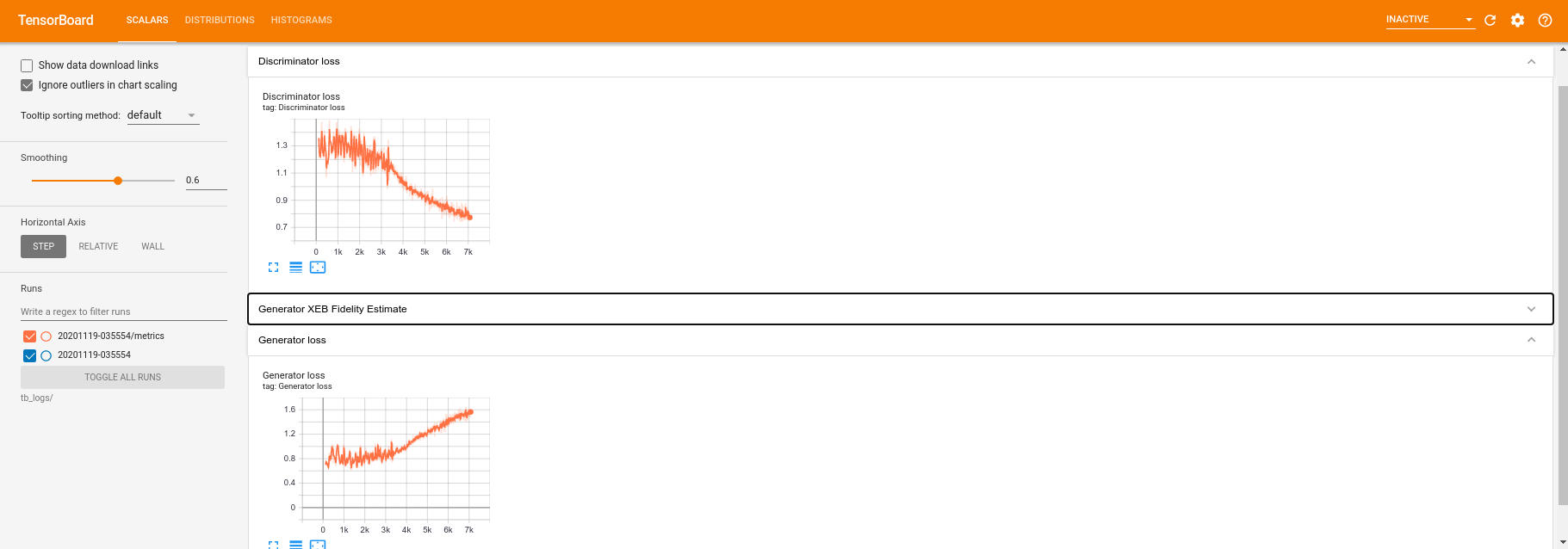
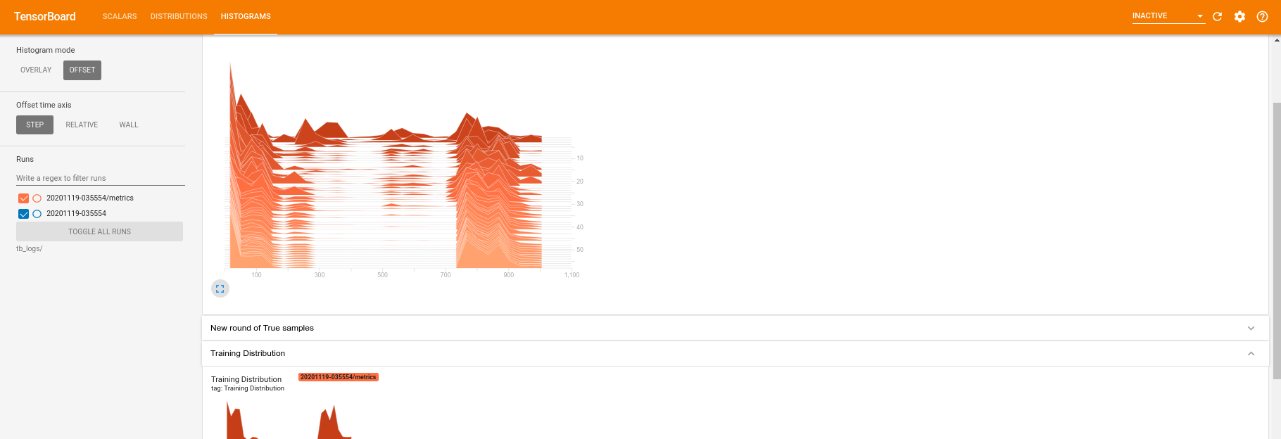
히스토그램 탭으로 전환하면 생성기 네트워크가 양자 분포에서 샘플을 재생성할 때 얼마나 잘 수행하는지 확인할 수도 있습니다.
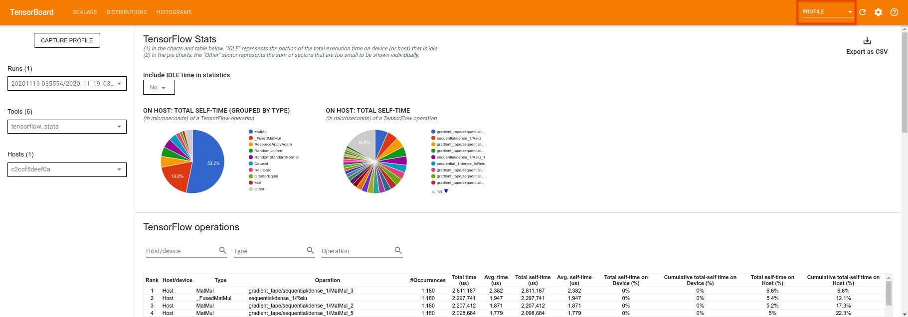
TensorBoard는 실험과 관련된 요약 통계의 실시간 모니터링을 허용하는 것 외에도 실험을 프로파일링하여 성능 병목 현상을 식별하는 데 도움을 줄 수 있습니다. 성능 모니터링으로 모델을 다시 실행하려면 다음을 수행할 수 있습니다.
tf.profiler.experimental.start(logdir)
train(all_data, epochs=10, start_epoch=50)
tf.profiler.experimental.stop()
Epoch 50, took 0.8879530429840088(s)
TensorBoard는 tf.profiler.experimental.start 와 tf.profiler.experimental.stop 사이의 모든 코드를 프로파일링합니다. 이 프로필 데이터는 TensorBoard의 profile 페이지에서 볼 수 있습니다.
깊이를 높이거나 다른 클래스의 양자 회로를 실험해 보십시오. TensorFlow Quantum 실험에 통합할 수 있는 초 매개변수 조정 과 같은 TensorBoard 의 다른 모든 훌륭한 기능을 확인하십시오.