
このチュートリアルでは、ディープラーニングを使用して、ある画像を別の画像の画風で作成します(ピカソやゴッホのように描いてみたいと思ったことはありませんか?)。これはニューラル画風変換として知られるテクニックで、「A Neural Algorithm of Artistic Style」(Gatys et al.)に説明されています。
注意: このチュートリアルでは、元の画風変換アルゴリズムを実演しています。画像のコンテンツを特定の画風に最適化するものです。最新のアプローチでは、画風が適用された画像を直接生成するようにモデルをトレーニングします(CycleGAN に類似)。このアプローチではより高速に実行することが可能です(最大 1000 倍)。
TensorFlow Hub から事前トレーニングされたモデルを使用した画風変換の簡単なアプリケーションについては、任意の画像様式化モデルを使用する任意のスタイルの高速画風変換のチュートリアルをご覧ください。TensorFlow Lite を使用した画風変換の例については、TensorFlow Lite を使用した芸術的な画風変換を参照してください。
ニューラル画風変換は、コンテンツ画像と画風参照画像(有名な画家の作品など)という 2 つの画像をブレンドしてコンテンツ画像に見えるが、画風参照画像の画風で「描かれた」ように見える画像を出力するための最適化テクニックです。
これは、コンテンツ画像のコンテンツ統計と画風参照画像の画風統計に一致するように出力画像を最適化することで実装されています。これらの統計は、畳み込みネットワークを使用して画像から抽出されます。
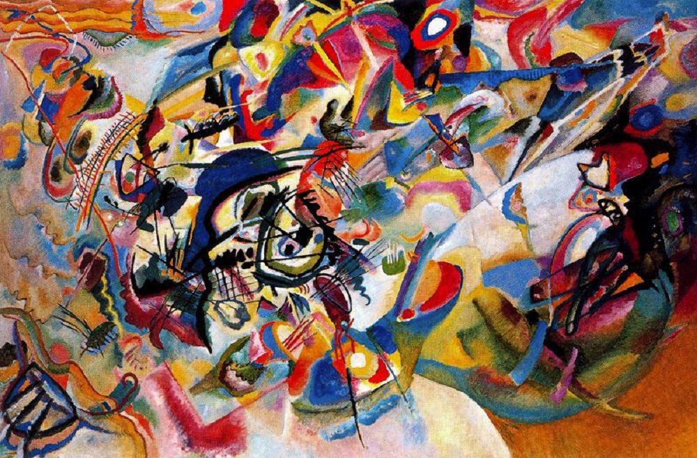
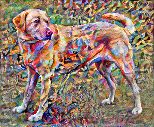
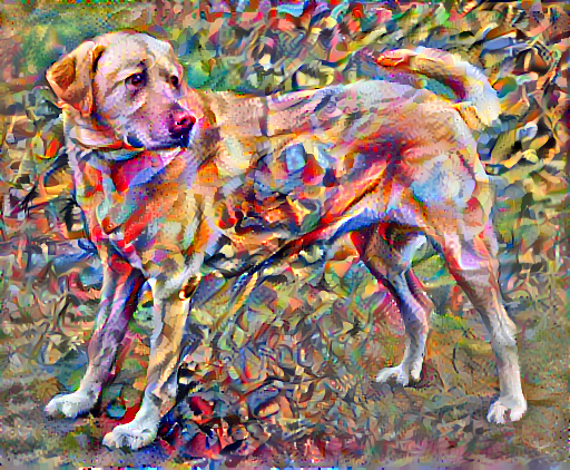
たとえば、以下の犬の画像とワシリー・カジンスキーの作品 7 を使用しましょう。
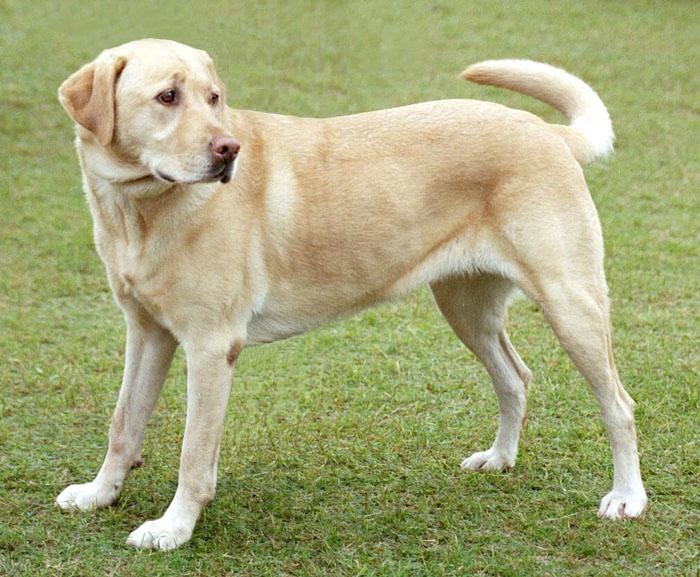
ウィキペディアコモンズの Yellow Labrador Looking。作成者、Elf。ライセンス CC BY-SA 3.0
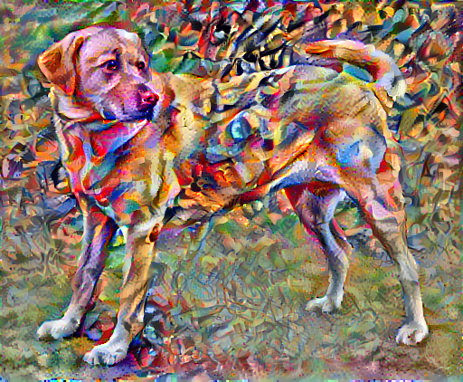
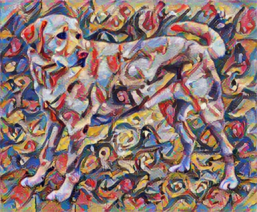
ガジンスキーがこの画風のみを使用してこの犬の絵を描こうとしたら、どのようになるのか見てみましょう。以下のようになるでしょうか?
セットアップ
モジュールのインポートと構成
import os
import tensorflow as tf
# Load compressed models from tensorflow_hub
os.environ['TFHUB_MODEL_LOAD_FORMAT'] = 'COMPRESSED'
2024-01-11 22:34:14.547246: E external/local_xla/xla/stream_executor/cuda/cuda_dnn.cc:9261] Unable to register cuDNN factory: Attempting to register factory for plugin cuDNN when one has already been registered
2024-01-11 22:34:14.547300: E external/local_xla/xla/stream_executor/cuda/cuda_fft.cc:607] Unable to register cuFFT factory: Attempting to register factory for plugin cuFFT when one has already been registered
2024-01-11 22:34:14.548982: E external/local_xla/xla/stream_executor/cuda/cuda_blas.cc:1515] Unable to register cuBLAS factory: Attempting to register factory for plugin cuBLAS when one has already been registered
import IPython.display as display

import matplotlib.pyplot as plt
import matplotlib as mpl
mpl.rcParams['figure.figsize'] = (12, 12)
mpl.rcParams['axes.grid'] = False

import numpy as np
import PIL.Image
import time
import functools
def tensor_to_image(tensor):
  tensor = tensor*255
  tensor = np.array(tensor, dtype=np.uint8)
  if np.ndim(tensor)>3:
    assert tensor.shape[0] == 1
    tensor = tensor[0]
  return PIL.Image.fromarray(tensor)
画像をダウンロードして、画風画像とコンテンツ画像を選択します。
content_path = tf.keras.utils.get_file('YellowLabradorLooking_new.jpg', 'https://storage.googleapis.com/download.tensorflow.org/example_images/YellowLabradorLooking_new.jpg')
style_path = tf.keras.utils.get_file('kandinsky5.jpg','https://storage.googleapis.com/download.tensorflow.org/example_images/Vassily_Kandinsky%2C_1913_-_Composition_7.jpg')
Downloading data from https://storage.googleapis.com/download.tensorflow.org/example_images/YellowLabradorLooking_new.jpg
83281/83281 [==============================] - 0s 0us/step
Downloading data from https://storage.googleapis.com/download.tensorflow.org/example_images/Vassily_Kandinsky%2C_1913_-_Composition_7.jpg
195196/195196 [==============================] - 0s 0us/step
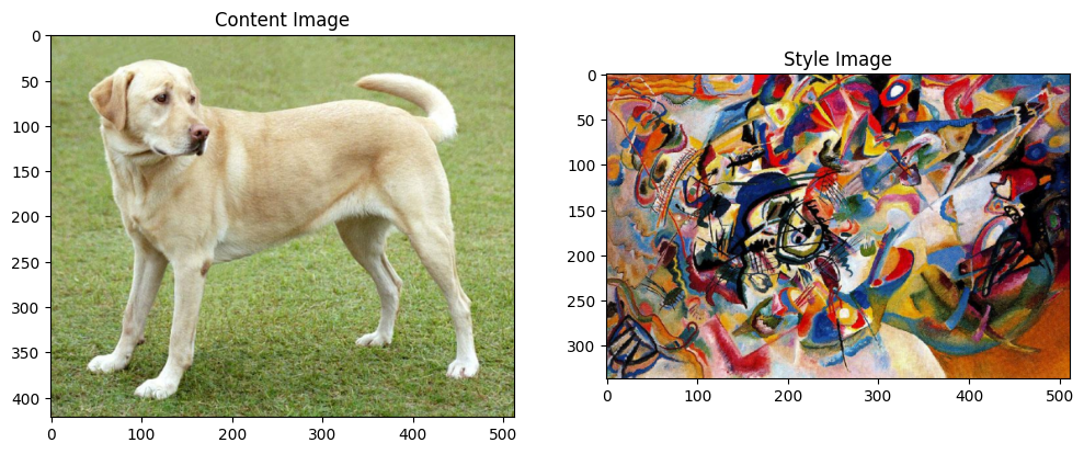
入力を視覚化する
画像を読み込んで、その最大寸法を 512 ピクセルに制限する関数を定義します。
def load_img(path_to_img):
  max_dim = 512
  img = tf.io.read_file(path_to_img)
  img = tf.image.decode_image(img, channels=3)
  img = tf.image.convert_image_dtype(img, tf.float32)

  shape = tf.cast(tf.shape(img)[:-1], tf.float32)
  long_dim = max(shape)
  scale = max_dim / long_dim

  new_shape = tf.cast(shape * scale, tf.int32)

  img = tf.image.resize(img, new_shape)
  img = img[tf.newaxis, :]
  return img
画像を表示する単純な関数を作成します。
def imshow(image, title=None):
  if len(image.shape) > 3:
    image = tf.squeeze(image, axis=0)

  plt.imshow(image)
  if title:
    plt.title(title)
content_image = load_img(content_path)
style_image = load_img(style_path)

plt.subplot(1, 2, 1)
imshow(content_image, 'Content Image')

plt.subplot(1, 2, 2)
imshow(style_image, 'Style Image')
TF-Hub を使用した高速画風変換
このチュートリアルでは、画像コンテンツを特定の画風に最適化する、元の画風変換アルゴリズムを実演します。詳細に踏み込む前に、TensorFlow Hub が何を行うのかを確認しましょう。
import tensorflow_hub as hub
hub_model = hub.load('https://tfhub.dev/google/magenta/arbitrary-image-stylization-v1-256/2')
stylized_image = hub_model(tf.constant(content_image), tf.constant(style_image))[0]
tensor_to_image(stylized_image)
コンテンツと画風の表現を定義する
モデルの中間レイヤーを使用して、画像のコンテンツと画風の表現を取得します。ネットワークの入力レイヤーから数えて最初のいくつかのレイヤーアクティベーションは、エッジやテクスチャといった低レベルの特徴を表します。ネットワークをさらに深く探ると、最後のいくつかのレイヤーは、車輪や目といった高レベルの特徴を表します。この場合、VGG19 ネットワークアーキテクチャという、事前トレーニング済みの画像分類ネットワークを使用しています。中間レイヤーは、画像からコンテンツと画風の表現を定義するために必要となるレイヤーです。入力画像については、これらの中間レイヤーにある、対応する画風とコンテンツターゲットの表現に一致するようにします。
VGG19 を読み込んで、画像で実行し、正しく使用されていることを確認します。
x = tf.keras.applications.vgg19.preprocess_input(content_image*255)
x = tf.image.resize(x, (224, 224))
vgg = tf.keras.applications.VGG19(include_top=True, weights='imagenet')
prediction_probabilities = vgg(x)
prediction_probabilities.shape
Downloading data from https://storage.googleapis.com/tensorflow/keras-applications/vgg19/vgg19_weights_tf_dim_ordering_tf_kernels.h5
574710816/574710816 [==============================] - 3s 0us/step
TensorShape([1, 1000])
predicted_top_5 = tf.keras.applications.vgg19.decode_predictions(prediction_probabilities.numpy())[0]
[(class_name, prob) for (number, class_name, prob) in predicted_top_5]
Downloading data from https://storage.googleapis.com/download.tensorflow.org/data/imagenet_class_index.json
35363/35363 [==============================] - 0s 0us/step
[('Labrador_retriever', 0.49317107),
 ('golden_retriever', 0.23665293),
 ('kuvasz', 0.03635751),
 ('Chesapeake_Bay_retriever', 0.024182767),
 ('Greater_Swiss_Mountain_dog', 0.018646102)]
分類ヘッドを除く VGG19 を読み込み、レイヤー名をリストします。
vgg = tf.keras.applications.VGG19(include_top=False, weights='imagenet')

print()
for layer in vgg.layers:
  print(layer.name)
Downloading data from https://storage.googleapis.com/tensorflow/keras-applications/vgg19/vgg19_weights_tf_dim_ordering_tf_kernels_notop.h5
80134624/80134624 [==============================] - 0s 0us/step

input_2
block1_conv1
block1_conv2
block1_pool
block2_conv1
block2_conv2
block2_pool
block3_conv1
block3_conv2
block3_conv3
block3_conv4
block3_pool
block4_conv1
block4_conv2
block4_conv3
block4_conv4
block4_pool
block5_conv1
block5_conv2
block5_conv3
block5_conv4
block5_pool
画像の画風とコンテンツを表現する中間レイヤーをネットワークから選択します。
content_layers = ['block5_conv2']

style_layers = ['block1_conv1',
                'block2_conv1',
                'block3_conv1',
                'block4_conv1',
                'block5_conv1']

num_content_layers = len(content_layers)
num_style_layers = len(style_layers)
画風とコンテンツ用の中間レイヤー
では、事前トレーニング済みの画像分類ネットワーク内のこれらの中間出力によって画風とコンテンツの表現を定義できるのはなぜでしょうか。
大まかに言えば、ネットワークが画像分類を行うには(このネットワークがトレーニングされた目的)、画像を理解している必要があります。これには、生の画像を入力ピクセルとして取り、生の画像ピクセルを、画像内に存在する特徴の複雑な理解への変換する内部表現が必要です。
これが、畳み込みニューラルネットワークがうまく一般化できる理由でもあります。不変性をキャプチャして、バックグラウンドノイズやその他の邪魔なものにとらわれない特徴をクラス内(猫と犬など)定義することができます。そのため、生の画像がモデルにフェードされる場所と出力分類ラベルの間のどこかで、モデルは複雑な特徴量抽出器としての役割を果たしていることになります。モデルの中間レイヤーにアクセスすることによって、入力画像のコンテンツと画風を説明することができます。
モデルを構築する
tf.keras.applications のネットワークは、Keras の Functional API を使用して、中間レイヤーの値を簡単に抽出できるように設計されています。
Functional API を使用してモデルを定義するには、入力と出力を以下のように指定します。
model = Model(inputs, outputs)
以下の関数は、中間レイヤーの出力を返す VGG19 モデルを構築します。
def vgg_layers(layer_names):
  """ Creates a VGG model that returns a list of intermediate output values."""
  # Load our model. Load pretrained VGG, trained on ImageNet data
  vgg = tf.keras.applications.VGG19(include_top=False, weights='imagenet')
  vgg.trainable = False

  outputs = [vgg.get_layer(name).output for name in layer_names]

  model = tf.keras.Model([vgg.input], outputs)
  return model
モデルを作成するには、以下のように行います。
style_extractor = vgg_layers(style_layers)
style_outputs = style_extractor(style_image*255)

#Look at the statistics of each layer's output
for name, output in zip(style_layers, style_outputs):
  print(name)
  print("  shape: ", output.numpy().shape)
  print("  min: ", output.numpy().min())
  print("  max: ", output.numpy().max())
  print("  mean: ", output.numpy().mean())
  print()
block1_conv1
  shape:  (1, 336, 512, 64)
  min:  0.0
  max:  835.5256
  mean:  33.97525

block2_conv1
  shape:  (1, 168, 256, 128)
  min:  0.0
  max:  4625.8857
  mean:  199.82687

block3_conv1
  shape:  (1, 84, 128, 256)
  min:  0.0
  max:  8789.239
  mean:  230.78099

block4_conv1
  shape:  (1, 42, 64, 512)
  min:  0.0
  max:  21566.135
  mean:  791.24005

block5_conv1
  shape:  (1, 21, 32, 512)
  min:  0.0
  max:  3189.2542
  mean:  59.179478
画風を計算する
画像のコンテンツは、中間特徴量マップの値によって表現されます。
これにより、画像の画風は、異なる特徴量マップの平均と相関によって表現できるようになります。各場所での特徴ベクトルの外積を取り、その外積をすべての場所で平均することにより、この情報を含むグラム行列を計算します。特定のレイヤーのグラム行列は以下のように計算できます。
これは、tf.linalg.einsum 関数を使用して、明確に実装することができます。
これは、 tf.linalg.einsum関数を使用して簡潔に実装できます。
def gram_matrix(input_tensor):
  result = tf.linalg.einsum('bijc,bijd->bcd', input_tensor, input_tensor)
  input_shape = tf.shape(input_tensor)
  num_locations = tf.cast(input_shape[1]*input_shape[2], tf.float32)
  return result/(num_locations)
画風とコンテンツを抽出する
画風とコンテンツのテンソルを返すモデルを構築します。
class StyleContentModel(tf.keras.models.Model):
  def __init__(self, style_layers, content_layers):
    super(StyleContentModel, self).__init__()
    self.vgg = vgg_layers(style_layers + content_layers)
    self.style_layers = style_layers
    self.content_layers = content_layers
    self.num_style_layers = len(style_layers)
    self.vgg.trainable = False

  def call(self, inputs):
    "Expects float input in [0,1]"
    inputs = inputs*255.0
    preprocessed_input = tf.keras.applications.vgg19.preprocess_input(inputs)
    outputs = self.vgg(preprocessed_input)
    style_outputs, content_outputs = (outputs[:self.num_style_layers],
                                      outputs[self.num_style_layers:])

    style_outputs = [gram_matrix(style_output)
                     for style_output in style_outputs]

    content_dict = {content_name: value
                    for content_name, value
                    in zip(self.content_layers, content_outputs)}

    style_dict = {style_name: value
                  for style_name, value
                  in zip(self.style_layers, style_outputs)}

    return {'content': content_dict, 'style': style_dict}
画像に対して呼び出されると、このモデルは style_layers のグラム行列(画風)と content_layers のコンテンツを返します。
extractor = StyleContentModel(style_layers, content_layers)

results = extractor(tf.constant(content_image))

print('Styles:')
for name, output in sorted(results['style'].items()):
  print("  ", name)
  print("    shape: ", output.numpy().shape)
  print("    min: ", output.numpy().min())
  print("    max: ", output.numpy().max())
  print("    mean: ", output.numpy().mean())
  print()

print("Contents:")
for name, output in sorted(results['content'].items()):
  print("  ", name)
  print("    shape: ", output.numpy().shape)
  print("    min: ", output.numpy().min())
  print("    max: ", output.numpy().max())
  print("    mean: ", output.numpy().mean())
Styles:
   block1_conv1
    shape:  (1, 64, 64)
    min:  0.005522845
    max:  28014.555
    mean:  263.79022

   block2_conv1
    shape:  (1, 128, 128)
    min:  0.0
    max:  61479.484
    mean:  9100.949

   block3_conv1
    shape:  (1, 256, 256)
    min:  0.0
    max:  545623.44
    mean:  7660.976

   block4_conv1
    shape:  (1, 512, 512)
    min:  0.0
    max:  4320502.0
    mean:  134288.84

   block5_conv1
    shape:  (1, 512, 512)
    min:  0.0
    max:  110005.37
    mean:  1487.0378

Contents:
   block5_conv2
    shape:  (1, 26, 32, 512)
    min:  0.0
    max:  2410.8796
    mean:  13.764149
勾配下降法を実行する
この画風とコンテンツの抽出器を使用して、画風変換アルゴリズムを実装できるようになりました。各ターゲットに相対する画像の出力の平均二乗誤差を計算し、これらの損失の加重和を取って行います。
画風とコンテンツターゲット値を設定します。
style_targets = extractor(style_image)['style']
content_targets = extractor(content_image)['content']
最適化する画像を含めて tf.Variable を定義します。これを素早く行うには、コンテンツ画像で初期化します(tf.Variable は、コンテンツ画像を同じ形状である必要があります)。
image = tf.Variable(content_image)
これはフローと画像であるため、ピクセル値を 0 から 1 に維持する関数を定義します。
def clip_0_1(image):
  return tf.clip_by_value(image, clip_value_min=0.0, clip_value_max=1.0)
オプティマイザを作成します。論文では、LBFGS が推奨されていますが、Adam も使用できます。
opt = tf.keras.optimizers.Adam(learning_rate=0.02, beta_1=0.99, epsilon=1e-1)
これを最適化するために、重みづけされた、2 つの損失の組み合わせを使用して合計損失を取得します。
style_weight=1e-2
content_weight=1e4
def style_content_loss(outputs):
    style_outputs = outputs['style']
    content_outputs = outputs['content']
    style_loss = tf.add_n([tf.reduce_mean((style_outputs[name]-style_targets[name])**2)
                           for name in style_outputs.keys()])
    style_loss *= style_weight / num_style_layers

    content_loss = tf.add_n([tf.reduce_mean((content_outputs[name]-content_targets[name])**2)
                             for name in content_outputs.keys()])
    content_loss *= content_weight / num_content_layers
    loss = style_loss + content_loss
    return loss
tf.GradientTape を使用して画像を更新します。
@tf.function()
def train_step(image):
  with tf.GradientTape() as tape:
    outputs = extractor(image)
    loss = style_content_loss(outputs)

  grad = tape.gradient(loss, image)
  opt.apply_gradients([(grad, image)])
  image.assign(clip_0_1(image))
いくつかのステップを実行してテストします。
train_step(image)
train_step(image)
train_step(image)
tensor_to_image(image)
WARNING: All log messages before absl::InitializeLog() is called are written to STDERR
I0000 00:00:1705012485.893139 1037644 device_compiler.h:186] Compiled cluster using XLA!  This line is logged at most once for the lifetime of the process.

機能しているので、さらに長い最適化を実行します。
import time
start = time.time()

epochs = 10
steps_per_epoch = 100

step = 0
for n in range(epochs):
  for m in range(steps_per_epoch):
    step += 1
    train_step(image)
    print(".", end='', flush=True)
  display.clear_output(wait=True)
  display.display(tensor_to_image(image))
  print("Train step: {}".format(step))

end = time.time()
print("Total time: {:.1f}".format(end-start))
Train step: 1000
Total time: 75.5
総変動損失
この基本実装には、 高周波アーチファクトが多く生成されるという難点があります。これらは、画像の高周波コンポーネントに明示的な正則化項を使用することで低下させることができます。画風変換では、通常これは総変動損失と呼ばれています。
def high_pass_x_y(image):
  x_var = image[:, :, 1:, :] - image[:, :, :-1, :]
  y_var = image[:, 1:, :, :] - image[:, :-1, :, :]

  return x_var, y_var
x_deltas, y_deltas = high_pass_x_y(content_image)

plt.figure(figsize=(14, 10))
plt.subplot(2, 2, 1)
imshow(clip_0_1(2*y_deltas+0.5), "Horizontal Deltas: Original")

plt.subplot(2, 2, 2)
imshow(clip_0_1(2*x_deltas+0.5), "Vertical Deltas: Original")

x_deltas, y_deltas = high_pass_x_y(image)

plt.subplot(2, 2, 3)
imshow(clip_0_1(2*y_deltas+0.5), "Horizontal Deltas: Styled")

plt.subplot(2, 2, 4)
imshow(clip_0_1(2*x_deltas+0.5), "Vertical Deltas: Styled")
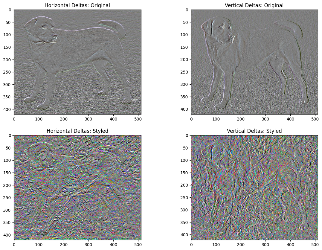
これは、高周波コンポーネントがどのように高まったのかを示します。
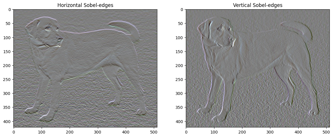
また、この高周波コンポーネントは基本的にエッジ検出器でもあります。似たような出力は、Sobel エッジ検出器でも見られます。以下に例を示します。
plt.figure(figsize=(14, 10))

sobel = tf.image.sobel_edges(content_image)
plt.subplot(1, 2, 1)
imshow(clip_0_1(sobel[..., 0]/4+0.5), "Horizontal Sobel-edges")
plt.subplot(1, 2, 2)
imshow(clip_0_1(sobel[..., 1]/4+0.5), "Vertical Sobel-edges")
これに伴う正則化損失は、値の二乗の和です。
def total_variation_loss(image):
  x_deltas, y_deltas = high_pass_x_y(image)
  return tf.reduce_sum(tf.abs(x_deltas)) + tf.reduce_sum(tf.abs(y_deltas))
total_variation_loss(image).numpy()
149329.9
何を行うかについては実演されましたが、これを自分で実装する必要はありません。TensorFlow には、標準実装が含まれています。
tf.image.total_variation(image).numpy()
array([149329.9], dtype=float32)
最適化を再実行する
total_variation_loss の重みを選択します。
total_variation_weight=30
train_step 関数にそれを含めます。
@tf.function()
def train_step(image):
  with tf.GradientTape() as tape:
    outputs = extractor(image)
    loss = style_content_loss(outputs)
    loss += total_variation_weight*tf.image.total_variation(image)

  grad = tape.gradient(loss, image)
  opt.apply_gradients([(grad, image)])
  image.assign(clip_0_1(image))
イメージ変数とオプティマイザーを再初期化します。
opt = tf.keras.optimizers.Adam(learning_rate=0.02, beta_1=0.99, epsilon=1e-1)
image = tf.Variable(content_image)
そして、最適化を実行します。
import time
start = time.time()

epochs = 10
steps_per_epoch = 100

step = 0
for n in range(epochs):
  for m in range(steps_per_epoch):
    step += 1
    train_step(image)
    print(".", end='', flush=True)
  display.clear_output(wait=True)
  display.display(tensor_to_image(image))
  print("Train step: {}".format(step))

end = time.time()
print("Total time: {:.1f}".format(end-start))
Train step: 1000
Total time: 82.2
最後に、結果を保存します。
file_name = 'stylized-image.png'
tensor_to_image(image).save(file_name)

try:
  from google.colab import files
except ImportError:
   pass
else:
  files.download(file_name)
詳細情報
このチュートリアルでは、元の画風変換アルゴリズムを紹介しました。画風変換の簡単なアプリケーションについては、このチュートリアルを参照してください。TensorFlow Hub から任意の画風変換モデルを使用する方法についての詳細が記載されています。