
| |
|
 GitHubでソースを表示 GitHubでソースを表示 |
このチュートリアルでは、MNIST の数の分類をするための、シンプルな畳み込みニューラルネットワーク (CNN: Convolutional Neural Network) の学習について説明します。このシンプルなネットワークは MNIST テストセットにおいて、99%以上の精度を達成します。このチュートリアルでは、Keras Sequential APIを使用するため、ほんの数行のコードでモデルの作成と学習を行うことができます。
Note: GPU を使うことで CNN をより早く学習させることができます。もし、このノートブックを Colab で実行しているならば、編集 -> ノートブックの設定 -> ハードウェアアクセラレータ -> GPU から無料のGPUを有効にすることができます。
TensorFlowのインポート
import tensorflow as tf

from tensorflow.keras import datasets, layers, models
import matplotlib.pyplot as plt
2024-01-11 22:25:45.947681: E external/local_xla/xla/stream_executor/cuda/cuda_dnn.cc:9261] Unable to register cuDNN factory: Attempting to register factory for plugin cuDNN when one has already been registered
2024-01-11 22:25:45.947724: E external/local_xla/xla/stream_executor/cuda/cuda_fft.cc:607] Unable to register cuFFT factory: Attempting to register factory for plugin cuFFT when one has already been registered
2024-01-11 22:25:45.949278: E external/local_xla/xla/stream_executor/cuda/cuda_blas.cc:1515] Unable to register cuBLAS factory: Attempting to register factory for plugin cuBLAS when one has already been registered
MNISTデータセットのダウンロードと準備
CIFAR10 データセットには、10 のクラスに 60,000 のカラー画像が含まれ、各クラスに 6,000 の画像が含まれています。 データセットは、50,000 のトレーニング画像と 10,000 のテスト画像に分割されています。クラスは相互に排他的であり、それらの間に重複はありません。
(train_images, train_labels), (test_images, test_labels) = datasets.cifar10.load_data()

# Normalize pixel values to be between 0 and 1
train_images, test_images = train_images / 255.0, test_images / 255.0
Downloading data from https://www.cs.toronto.edu/~kriz/cifar-10-python.tar.gz
170498071/170498071 [==============================] - 2s 0us/step
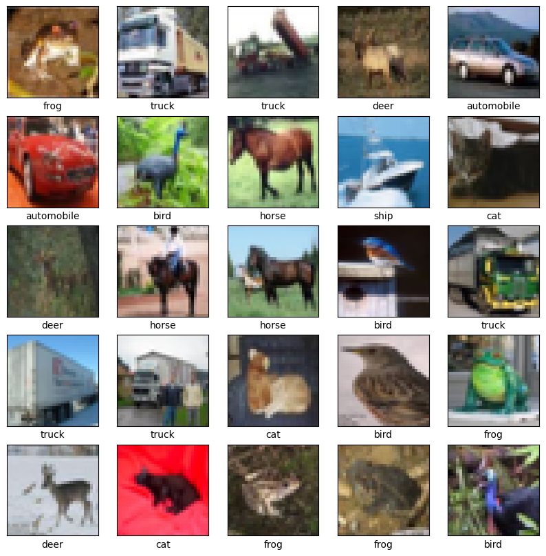
データを確認する
データセットが正しいことを確認するために、トレーニングセットの最初の 25 枚の画像をプロットし、各画像の下にクラス名を表示しましょう。
class_names = ['airplane', 'automobile', 'bird', 'cat', 'deer',
               'dog', 'frog', 'horse', 'ship', 'truck']

plt.figure(figsize=(10,10))
for i in range(25):
    plt.subplot(5,5,i+1)
    plt.xticks([])
    plt.yticks([])
    plt.grid(False)
    plt.imshow(train_images[i])
    # The CIFAR labels happen to be arrays,
    # which is why you need the extra index
    plt.xlabel(class_names[train_labels[i][0]])
plt.show()
畳み込みの基礎部分の作成
下記の6行のコードは、一般的なパターンで畳み込みの基礎部分を定義しています: Conv2D と MaxPooling2D レイヤーのスタック。
入力として、CNNはバッチサイズを無視して、形状(image_height、image_width、color_channels)のテンソルを取ります。これらのディメンションを初めて使用する場合、color_channelsは(R,G,B)を参照します。 この例では、CIFAR 画像の形式である形状(32, 32, 3)の入力を処理するようにCNNを構成します。これを行うには、引数input_shapeを最初のレイヤーに渡します。
model = models.Sequential()
model.add(layers.Conv2D(32, (3, 3), activation='relu', input_shape=(32, 32, 3)))
model.add(layers.MaxPooling2D((2, 2)))
model.add(layers.Conv2D(64, (3, 3), activation='relu'))
model.add(layers.MaxPooling2D((2, 2)))
model.add(layers.Conv2D(64, (3, 3), activation='relu'))
これまでのモデルのアーキテクチャを表示します。
model.summary()
Model: "sequential"
_________________________________________________________________
 Layer (type)                Output Shape              Param #
=================================================================
 conv2d (Conv2D)             (None, 30, 30, 32)        896

 max_pooling2d (MaxPooling2  (None, 15, 15, 32)        0
 D)

 conv2d_1 (Conv2D)           (None, 13, 13, 64)        18496

 max_pooling2d_1 (MaxPoolin  (None, 6, 6, 64)          0
 g2D)

 conv2d_2 (Conv2D)           (None, 4, 4, 64)          36928

=================================================================
Total params: 56320 (220.00 KB)
Trainable params: 56320 (220.00 KB)
Non-trainable params: 0 (0.00 Byte)
_________________________________________________________________
上記より、すべての Conv2D と MaxPooling2D レイヤーの出力は shape (height, width, channels) の 3D テンソルであることがわかります。width と height の寸法は、ネットワークが深くなるにつれて縮小する傾向があります。各 Conv2D レイヤーの出力チャネルの数は、第一引数 (例: 32 または 64) によって制御されます。通常、width とheight が縮小すると、各 Conv2D レイヤーにさらに出力チャネルを追加する余裕が (計算上) できます。
上に Dense レイヤーを追加
モデルを完成するために、(shape (3, 3, 64) の) 畳み込みの基礎部分からの最後の出力テンソルを、1つ以上の Dense レイヤーに入れて分類を実行します。現在の出力は 3D テンソルですが、Dense レイヤーは入力としてベクトル (1D) を取ります。まず、3D 出力を 1D に平滑化 (または展開) してから、最上部に1つ以上の Dense レイヤーを追加します。MNIST は 10 個の出力クラスを持ちます。そのため、我々は最後の Dense レイヤーの出力を 10 にし、softmax関数を使用します。
model.add(layers.Flatten())
model.add(layers.Dense(64, activation='relu'))
model.add(layers.Dense(10))
モデルの完全なアーキテクチャは次のとおりです。
model.summary()
Model: "sequential"
_________________________________________________________________
 Layer (type)                Output Shape              Param #
=================================================================
 conv2d (Conv2D)             (None, 30, 30, 32)        896

 max_pooling2d (MaxPooling2  (None, 15, 15, 32)        0
 D)

 conv2d_1 (Conv2D)           (None, 13, 13, 64)        18496

 max_pooling2d_1 (MaxPoolin  (None, 6, 6, 64)          0
 g2D)

 conv2d_2 (Conv2D)           (None, 4, 4, 64)          36928

 flatten (Flatten)           (None, 1024)              0

 dense (Dense)               (None, 64)                65600

 dense_1 (Dense)             (None, 10)                650

=================================================================
Total params: 122570 (478.79 KB)
Trainable params: 122570 (478.79 KB)
Non-trainable params: 0 (0.00 Byte)
_________________________________________________________________
ネットワークの要約は、(4, 4, 64) 出力が、2 つの高密度レイヤーを通過する前に形状のベクトル (1024) に平坦化されたことを示しています。
モデルのコンパイルと学習
model.compile(optimizer='adam',
              loss=tf.keras.losses.SparseCategoricalCrossentropy(from_logits=True),
              metrics=['accuracy'])

history = model.fit(train_images, train_labels, epochs=10,
                    validation_data=(test_images, test_labels))
Epoch 1/10
WARNING: All log messages before absl::InitializeLog() is called are written to STDERR
I0000 00:00:1705011960.257626 1026150 device_compiler.h:186] Compiled cluster using XLA!  This line is logged at most once for the lifetime of the process.
1563/1563 [==============================] - 10s 5ms/step - loss: 1.5172 - accuracy: 0.4479 - val_loss: 1.2221 - val_accuracy: 0.5568
Epoch 2/10
1563/1563 [==============================] - 6s 4ms/step - loss: 1.1550 - accuracy: 0.5909 - val_loss: 1.0829 - val_accuracy: 0.6153
Epoch 3/10
1563/1563 [==============================] - 6s 4ms/step - loss: 1.0217 - accuracy: 0.6406 - val_loss: 1.0480 - val_accuracy: 0.6356
Epoch 4/10
1563/1563 [==============================] - 6s 4ms/step - loss: 0.9275 - accuracy: 0.6763 - val_loss: 0.9510 - val_accuracy: 0.6671
Epoch 5/10
1563/1563 [==============================] - 6s 4ms/step - loss: 0.8631 - accuracy: 0.6983 - val_loss: 0.9596 - val_accuracy: 0.6608
Epoch 6/10
1563/1563 [==============================] - 6s 4ms/step - loss: 0.8053 - accuracy: 0.7187 - val_loss: 0.9203 - val_accuracy: 0.6798
Epoch 7/10
1563/1563 [==============================] - 6s 4ms/step - loss: 0.7594 - accuracy: 0.7338 - val_loss: 0.8939 - val_accuracy: 0.6889
Epoch 8/10
1563/1563 [==============================] - 6s 4ms/step - loss: 0.7149 - accuracy: 0.7503 - val_loss: 0.8601 - val_accuracy: 0.6980
Epoch 9/10
1563/1563 [==============================] - 6s 4ms/step - loss: 0.6745 - accuracy: 0.7633 - val_loss: 0.8770 - val_accuracy: 0.6984
Epoch 10/10
1563/1563 [==============================] - 7s 4ms/step - loss: 0.6391 - accuracy: 0.7736 - val_loss: 0.8815 - val_accuracy: 0.7013
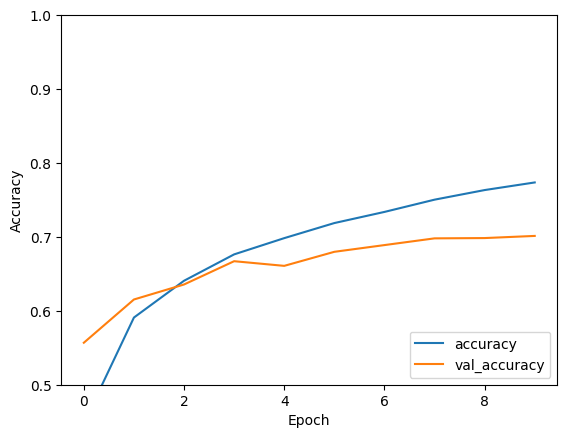
モデルの評価
plt.plot(history.history['accuracy'], label='accuracy')
plt.plot(history.history['val_accuracy'], label = 'val_accuracy')
plt.xlabel('Epoch')
plt.ylabel('Accuracy')
plt.ylim([0.5, 1])
plt.legend(loc='lower right')

test_loss, test_acc = model.evaluate(test_images,  test_labels, verbose=2)
313/313 - 1s - loss: 0.8815 - accuracy: 0.7013 - 676ms/epoch - 2ms/step
print(test_acc)
0.7013000249862671
この単純な CNN は、 数行のコードで 70% を超えるテスト精度を達成しています。別の CNN スタイルについては、Keras サブクラス化 API と{tf.GradientTapeを使用する 上級者向け TensorFlow 2 クイックスタートの例を参照してください。