
| | |  ดูแหล่งที่มาบน GitHub ดูแหล่งที่มาบน GitHub |
โน๊ตบุ๊คนี้รถไฟลำดับลำดับ (seq2seq) แบบจำลองสำหรับสเปนแปลเป็นภาษาอังกฤษขึ้นอยู่กับการ มีผลบังคับใช้แนวทางการเรียนตามประสาทเครื่องแปลภาษา นี่เป็นตัวอย่างขั้นสูงที่ถือว่ามีความรู้เกี่ยวกับ:
- ลำดับของแบบจำลองลำดับ
- พื้นฐาน TensorFlow ใต้เลเยอร์ keras:
- การทำงานกับเทนเซอร์โดยตรง
- การเขียนแบบกำหนดเอง
keras.Modelและkeras.layers
ในขณะที่สถาปัตยกรรมนี้จะล้าสมัยไปบ้างก็ยังคงเป็นโครงการที่มีประโยชน์มากในการทำงานผ่านไปได้รับความรู้ความเข้าใจในกลไกความสนใจ (ก่อนที่จะ Transformers )
หลังจากการฝึกอบรมรุ่นในสมุดบันทึกนี้คุณจะสามารถที่จะใส่ประโยคภาษาสเปนเช่นและกลับแปลภาษาอังกฤษ "¿ todavia estan en Casa?": "คุณยังคงอยู่ที่บ้าน"
รูปแบบที่เกิดเป็นที่ส่งสินค้าออกเป็น tf.saved_model เพื่อที่จะสามารถนำมาใช้ในสภาพแวดล้อมที่ TensorFlow อื่น ๆ
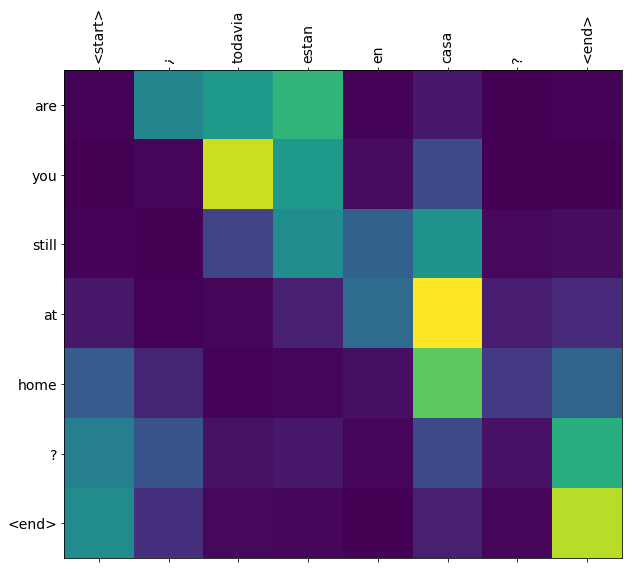
คุณภาพการแปลมีความสมเหตุสมผลสำหรับตัวอย่างของเล่น แต่พล็อตความสนใจที่สร้างขึ้นอาจมีความน่าสนใจมากกว่า นี่แสดงให้เห็นว่าส่วนใดของประโยคอินพุตที่มีความสนใจของนางแบบขณะแปล:
ติดตั้ง
pip install tensorflow_text
import numpy as np

import typing
from typing import Any, Tuple

import tensorflow as tf

import tensorflow_text as tf_text

import matplotlib.pyplot as plt
import matplotlib.ticker as ticker
บทช่วยสอนนี้สร้างเลเยอร์สองสามชั้นตั้งแต่เริ่มต้น ใช้ตัวแปรนี้หากคุณต้องการสลับไปมาระหว่างการใช้งานแบบกำหนดเองและในตัว
use_builtins = True
บทช่วยสอนนี้ใช้ API ระดับต่ำจำนวนมากซึ่งทำให้ง่ายต่อการเข้าใจผิด คลาสนี้ใช้ตรวจสอบรูปร่างตลอดบทช่วยสอน
ตัวตรวจสอบรูปร่าง
class ShapeChecker():
  def __init__(self):
    # Keep a cache of every axis-name seen
    self.shapes = {}

  def __call__(self, tensor, names, broadcast=False):
    if not tf.executing_eagerly():
      return

    if isinstance(names, str):
      names = (names,)

    shape = tf.shape(tensor)
    rank = tf.rank(tensor)

    if rank != len(names):
      raise ValueError(f'Rank mismatch:\n'
                       f'    found {rank}: {shape.numpy()}\n'
                       f'    expected {len(names)}: {names}\n')

    for i, name in enumerate(names):
      if isinstance(name, int):
        old_dim = name
      else:
        old_dim = self.shapes.get(name, None)
      new_dim = shape[i]

      if (broadcast and new_dim == 1):
        continue

      if old_dim is None:
        # If the axis name is new, add its length to the cache.
        self.shapes[name] = new_dim
        continue

      if new_dim != old_dim:
        raise ValueError(f"Shape mismatch for dimension: '{name}'\n"
                         f"    found: {new_dim}\n"
                         f"    expected: {old_dim}\n")
ข้อมูล
เราจะใช้ชุดภาษาให้โดย http://www.manythings.org/anki/ ชุดนี้มีคู่แปลภาษาในรูปแบบ:
May I borrow this book? ¿Puedo tomar prestado este libro?
มีหลายภาษาให้เลือก แต่เราจะใช้ชุดข้อมูลภาษาอังกฤษ-สเปน
ดาวน์โหลดและเตรียมชุดข้อมูล
เพื่อความสะดวก เราได้โฮสต์สำเนาของชุดข้อมูลนี้บน Google Cloud แต่คุณสามารถดาวน์โหลดสำเนาของคุณเองได้เช่นกัน หลังจากดาวน์โหลดชุดข้อมูลแล้ว ต่อไปนี้คือขั้นตอนที่เราจะดำเนินการเพื่อเตรียมข้อมูล:
- เพิ่มเริ่มต้นและสิ้นสุดโทเค็นแต่ละประโยค
- ทำความสะอาดประโยคโดยลบอักขระพิเศษ
- สร้างดัชนีคำและดัชนีคำย้อนกลับ (การทำแผนที่พจนานุกรมจาก word → id และ id → word)
- ปาดแต่ละประโยคให้มีความยาวสูงสุด
# Download the file
import pathlib

path_to_zip = tf.keras.utils.get_file(
    'spa-eng.zip', origin='http://storage.googleapis.com/download.tensorflow.org/data/spa-eng.zip',
    extract=True)

path_to_file = pathlib.Path(path_to_zip).parent/'spa-eng/spa.txt'
Downloading data from http://storage.googleapis.com/download.tensorflow.org/data/spa-eng.zip
2646016/2638744 [==============================] - 0s 0us/step
2654208/2638744 [==============================] - 0s 0us/step
def load_data(path):
  text = path.read_text(encoding='utf-8')

  lines = text.splitlines()
  pairs = [line.split('\t') for line in lines]

  inp = [inp for targ, inp in pairs]
  targ = [targ for targ, inp in pairs]

  return targ, inp
targ, inp = load_data(path_to_file)
print(inp[-1])
Si quieres sonar como un hablante nativo, debes estar dispuesto a practicar diciendo la misma frase una y otra vez de la misma manera en que un músico de banjo practica el mismo fraseo una y otra vez hasta que lo puedan tocar correctamente y en el tiempo esperado.
print(targ[-1])
If you want to sound like a native speaker, you must be willing to practice saying the same sentence over and over in the same way that banjo players practice the same phrase over and over until they can play it correctly and at the desired tempo.
สร้างชุดข้อมูล tf.data
จากอาร์เรย์เหล่านี้ของสตริงคุณสามารถสร้าง tf.data.Dataset ของสตริงที่ฟืดและแบตช์พวกเขาได้อย่างมีประสิทธิภาพ:
BUFFER_SIZE = len(inp)
BATCH_SIZE = 64

dataset = tf.data.Dataset.from_tensor_slices((inp, targ)).shuffle(BUFFER_SIZE)
dataset = dataset.batch(BATCH_SIZE)
for example_input_batch, example_target_batch in dataset.take(1):
  print(example_input_batch[:5])
  print()
  print(example_target_batch[:5])
  break
tf.Tensor(
[b'No s\xc3\xa9 lo que quiero.' b'\xc2\xbfDeber\xc3\xada repetirlo?'
 b'Tard\xc3\xa9 m\xc3\xa1s de 2 horas en traducir unas p\xc3\xa1ginas en ingl\xc3\xa9s.'
 b'A Tom comenz\xc3\xb3 a temerle a Mary.' b'Mi pasatiempo es la lectura.'], shape=(5,), dtype=string)

tf.Tensor(
[b"I don't know what I want." b'Should I repeat it?'
 b'It took me more than two hours to translate a few pages of English.'
 b'Tom became afraid of Mary.' b'My hobby is reading.'], shape=(5,), dtype=string)
การประมวลผลข้อความล่วงหน้า
หนึ่งในเป้าหมายของการกวดวิชานี้คือการสร้างรูปแบบที่สามารถส่งออกเป็นที่ tf.saved_model ที่จะทำให้รูปแบบการส่งออกที่มีประโยชน์จึงควรใช้ tf.string ปัจจัยการผลิตและส่งกลับ tf.string เอาท์พุท: ทั้งหมดการประมวลผลข้อความที่เกิดขึ้นภายในรูปแบบ
มาตรฐาน
โมเดลนี้จะจัดการกับข้อความหลายภาษาที่มีคำศัพท์จำกัด ดังนั้นจึงเป็นเรื่องสำคัญที่จะต้องกำหนดมาตรฐานของข้อความที่ป้อน
ขั้นตอนแรกคือการทำให้เป็นมาตรฐาน Unicode เพื่อแยกอักขระเน้นเสียงและแทนที่อักขระที่เข้ากันได้ด้วยการเทียบเท่า ASCII
tensorflow_text แพคเกจประกอบด้วยการดำเนินการ Unicode ปกติ:
example_text = tf.constant('¿Todavía está en casa?')

print(example_text.numpy())
print(tf_text.normalize_utf8(example_text, 'NFKD').numpy())
b'\xc2\xbfTodav\xc3\xada est\xc3\xa1 en casa?'
b'\xc2\xbfTodavi\xcc\x81a esta\xcc\x81 en casa?'
การทำให้เป็นมาตรฐาน Unicode จะเป็นขั้นตอนแรกในฟังก์ชันมาตรฐานข้อความ:
def tf_lower_and_split_punct(text):
  # Split accecented characters.
  text = tf_text.normalize_utf8(text, 'NFKD')
  text = tf.strings.lower(text)
  # Keep space, a to z, and select punctuation.
  text = tf.strings.regex_replace(text, '[^ a-z.?!,¿]', '')
  # Add spaces around punctuation.
  text = tf.strings.regex_replace(text, '[.?!,¿]', r' \0 ')
  # Strip whitespace.
  text = tf.strings.strip(text)

  text = tf.strings.join(['[START]', text, '[END]'], separator=' ')
  return text
print(example_text.numpy().decode())
print(tf_lower_and_split_punct(example_text).numpy().decode())
¿Todavía está en casa?
[START] ¿ todavia esta en casa ? [END]
การแปลงข้อความเป็นเวกเตอร์
ฟังก์ชั่นมาตรฐานนี้จะถูกห่อขึ้นใน tf.keras.layers.TextVectorization ชั้นซึ่งจะจัดการกับการสกัดคำศัพท์และการเปลี่ยนแปลงของการป้อนข้อความลำดับของสัญญาณ
max_vocab_size = 5000

input_text_processor = tf.keras.layers.TextVectorization(
    standardize=tf_lower_and_split_punct,
    max_tokens=max_vocab_size)
TextVectorization ชั้นและหลายชั้นก่อนการประมวลผลอื่น ๆ มีการ adapt วิธีการ วิธีการนี้อ่านหนึ่งยุคของข้อมูลการฝึกอบรมและการทำงานจำนวนมากเช่น Model.fix นี้ adapt วิธีการเริ่มต้นชั้นบนพื้นฐานของข้อมูล ที่นี่กำหนดคำศัพท์:
input_text_processor.adapt(inp)

# Here are the first 10 words from the vocabulary:
input_text_processor.get_vocabulary()[:10]
['', '[UNK]', '[START]', '[END]', '.', 'que', 'de', 'el', 'a', 'no']
นั่นคือสเปน TextVectorization ชั้นตอนนี้สร้างและ .adapt() ภาษาอังกฤษที่หนึ่ง:
output_text_processor = tf.keras.layers.TextVectorization(
    standardize=tf_lower_and_split_punct,
    max_tokens=max_vocab_size)

output_text_processor.adapt(targ)
output_text_processor.get_vocabulary()[:10]
['', '[UNK]', '[START]', '[END]', '.', 'the', 'i', 'to', 'you', 'tom']
ตอนนี้เลเยอร์เหล่านี้สามารถแปลงชุดของสตริงเป็นชุดของรหัสโทเค็น:
example_tokens = input_text_processor(example_input_batch)
example_tokens[:3, :10]
<tf.Tensor: shape=(3, 10), dtype=int64, numpy=
array([[   2,    9,   17,   22,    5,   48,    4,    3,    0,    0],
       [   2,   13,  177,    1,   12,    3,    0,    0,    0,    0],
       [   2,  120,   35,    6,  290,   14, 2134,  506, 2637,   14]])>
get_vocabulary วิธีการที่สามารถใช้ในการแปลงรหัสโทเค็นกลับไปเป็นข้อความ:
input_vocab = np.array(input_text_processor.get_vocabulary())
tokens = input_vocab[example_tokens[0].numpy()]
' '.join(tokens)
'[START] no se lo que quiero . [END] '
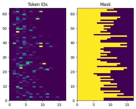
รหัสโทเค็นที่ส่งคืนนั้นเป็นศูนย์ นี้สามารถเปลี่ยนเป็นหน้ากากได้อย่างง่ายดาย:
plt.subplot(1, 2, 1)
plt.pcolormesh(example_tokens)
plt.title('Token IDs')

plt.subplot(1, 2, 2)
plt.pcolormesh(example_tokens != 0)
plt.title('Mask')
Text(0.5, 1.0, 'Mask')
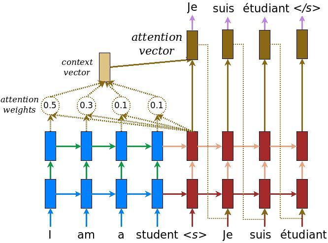
ตัวเข้ารหัส/ตัวถอดรหัส
ไดอะแกรมต่อไปนี้แสดงภาพรวมของโมเดล ในแต่ละขั้นตอนของเวลา เอาต์พุตของตัวถอดรหัสจะรวมกับผลรวมถ่วงน้ำหนักเหนืออินพุตที่เข้ารหัส เพื่อทำนายคำถัดไป แผนภาพและสูตรจาก กระดาษ Luong ของ
ก่อนที่จะเข้าไป ให้กำหนดค่าคงที่สองสามตัวสำหรับโมเดล:
embedding_dim = 256
units = 1024
ตัวเข้ารหัส
เริ่มต้นด้วยการสร้างตัวเข้ารหัส ซึ่งเป็นส่วนสีน้ำเงินของไดอะแกรมด้านบน
ตัวเข้ารหัส:
- นำรายการรหัสสัญญาณ (จาก
input_text_processor) - เงยหน้าขึ้นมองเวกเตอร์ฝังสำหรับแต่ละโทเค็น (ใช้
layers.Embedding) - กระบวนการ embeddings เป็นลำดับใหม่ (ใช้
layers.GRU) - ผลตอบแทน:
- ลำดับการประมวลผล นี้จะถูกส่งต่อไปยังหัวความสนใจ
- สภาพภายใน. สิ่งนี้จะถูกใช้เพื่อเริ่มต้นตัวถอดรหัส
class Encoder(tf.keras.layers.Layer):
  def __init__(self, input_vocab_size, embedding_dim, enc_units):
    super(Encoder, self).__init__()
    self.enc_units = enc_units
    self.input_vocab_size = input_vocab_size

    # The embedding layer converts tokens to vectors
    self.embedding = tf.keras.layers.Embedding(self.input_vocab_size,
                                               embedding_dim)

    # The GRU RNN layer processes those vectors sequentially.
    self.gru = tf.keras.layers.GRU(self.enc_units,
                                   # Return the sequence and state
                                   return_sequences=True,
                                   return_state=True,
                                   recurrent_initializer='glorot_uniform')

  def call(self, tokens, state=None):
    shape_checker = ShapeChecker()
    shape_checker(tokens, ('batch', 's'))

    # 2. The embedding layer looks up the embedding for each token.
    vectors = self.embedding(tokens)
    shape_checker(vectors, ('batch', 's', 'embed_dim'))

    # 3. The GRU processes the embedding sequence.
    #    output shape: (batch, s, enc_units)
    #    state shape: (batch, enc_units)
    output, state = self.gru(vectors, initial_state=state)
    shape_checker(output, ('batch', 's', 'enc_units'))
    shape_checker(state, ('batch', 'enc_units'))

    # 4. Returns the new sequence and its state.
    return output, state
นี่คือวิธีที่มันเข้ากันได้ดี:
# Convert the input text to tokens.
example_tokens = input_text_processor(example_input_batch)

# Encode the input sequence.
encoder = Encoder(input_text_processor.vocabulary_size(),
                  embedding_dim, units)
example_enc_output, example_enc_state = encoder(example_tokens)

print(f'Input batch, shape (batch): {example_input_batch.shape}')
print(f'Input batch tokens, shape (batch, s): {example_tokens.shape}')
print(f'Encoder output, shape (batch, s, units): {example_enc_output.shape}')
print(f'Encoder state, shape (batch, units): {example_enc_state.shape}')
Input batch, shape (batch): (64,)
Input batch tokens, shape (batch, s): (64, 14)
Encoder output, shape (batch, s, units): (64, 14, 1024)
Encoder state, shape (batch, units): (64, 1024)
ตัวเข้ารหัสจะส่งคืนสถานะภายในเพื่อให้สามารถใช้สถานะเพื่อเริ่มต้นตัวถอดรหัสได้
เป็นเรื่องปกติที่ RNN จะคืนค่าสถานะเพื่อให้สามารถประมวลผลลำดับผ่านการเรียกหลาย ๆ ครั้งได้ คุณจะเห็นการสร้างตัวถอดรหัสมากขึ้น
หัวความสนใจ
ตัวถอดรหัสใช้ความสนใจเพื่อเลือกโฟกัสที่ส่วนต่างๆ ของลำดับอินพุต ความสนใจจะใช้ลำดับของเวกเตอร์เป็นอินพุตสำหรับแต่ละตัวอย่าง และส่งกลับเวกเตอร์ "ความสนใจ" สำหรับแต่ละตัวอย่าง ชั้นความสนใจนี้จะคล้ายกับ layers.GlobalAveragePoling1D แต่ชั้นความสนใจดำเนินการถัวเฉลี่ยถ่วงน้ำหนัก
มาดูกันว่ามันทำงานอย่างไร:


ที่ไหน:
- \(s\) เป็นดัชนีการเข้ารหัส
- \(t\) ดัชนีถอดรหัส
- \(\alpha_{ts}\) เป็นน้ำหนักความสนใจ
- \(h_s\) เป็นลำดับของผลการเข้ารหัสที่มีการเข้าร่วม (ความสนใจ "ที่สำคัญ" และ "ค่า" ในคำศัพท์หม้อแปลง)
- \(h_t\) เป็นรัฐถอดรหัสการเข้าร่วมการลำดับ (ความสนใจ "แบบสอบถาม" ในคำศัพท์หม้อแปลง)
- \(c_t\) เป็นผลเวกเตอร์บริบท
- \(a_t\) เป็นผลลัพธ์สุดท้ายรวม "บริบท" และ "แบบสอบถาม"
สมการ:
- คำนวณความสนใจน้ำหนัก \(\alpha_{ts}\)เป็น softmax ข้ามลำดับผลผลิตเข้ารหัสไว้
- คำนวณเวกเตอร์บริบทเป็นผลรวมถ่วงน้ำหนักของเอาต์พุตตัวเข้ารหัส
สุดท้ายคือ \(score\) ฟังก์ชั่น หน้าที่ของมันคือการคำนวณคะแนนบันทึกสเกลาร์สำหรับคู่การสืบค้นคีย์แต่ละคู่ มีสองแนวทางทั่วไป:
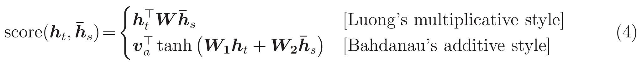
กวดวิชานี้จะใช้ ความสนใจของสารเติมแต่ง Bahdanau ของ TensorFlow รวมถึงการใช้งานของทั้งสองเป็น layers.Attention และ layers.AdditiveAttention ชั้นด้านล่างจับเมทริกซ์น้ำหนักในคู่ของ layers.Dense เลเยอร์และเรียกร้องให้ดำเนินการ builtin
class BahdanauAttention(tf.keras.layers.Layer):
  def __init__(self, units):
    super().__init__()
    # For Eqn. (4), the  Bahdanau attention
    self.W1 = tf.keras.layers.Dense(units, use_bias=False)
    self.W2 = tf.keras.layers.Dense(units, use_bias=False)

    self.attention = tf.keras.layers.AdditiveAttention()

  def call(self, query, value, mask):
    shape_checker = ShapeChecker()
    shape_checker(query, ('batch', 't', 'query_units'))
    shape_checker(value, ('batch', 's', 'value_units'))
    shape_checker(mask, ('batch', 's'))

    # From Eqn. (4), `W1@ht`.
    w1_query = self.W1(query)
    shape_checker(w1_query, ('batch', 't', 'attn_units'))

    # From Eqn. (4), `W2@hs`.
    w2_key = self.W2(value)
    shape_checker(w2_key, ('batch', 's', 'attn_units'))

    query_mask = tf.ones(tf.shape(query)[:-1], dtype=bool)
    value_mask = mask

    context_vector, attention_weights = self.attention(
        inputs = [w1_query, value, w2_key],
        mask=[query_mask, value_mask],
        return_attention_scores = True,
    )
    shape_checker(context_vector, ('batch', 't', 'value_units'))
    shape_checker(attention_weights, ('batch', 't', 's'))

    return context_vector, attention_weights
ทดสอบ Attention layer
สร้าง BahdanauAttention ชั้น:
attention_layer = BahdanauAttention(units)
เลเยอร์นี้รับ 3 อินพุต:
-
queryนี้จะถูกสร้างขึ้นโดยถอดรหัสภายหลัง -
value: นี่จะเป็นผลลัพธ์ของการเข้ารหัสที่ -
mask: หากต้องการยกเว้นช่องว่างภายใน,example_tokens != 0
(example_tokens != 0).shape
TensorShape([64, 14])
การนำเลเยอร์ความสนใจไปใช้แบบเวคเตอร์ทำให้คุณสามารถส่งชุดของลำดับของเวกเตอร์การสืบค้นและชุดของลำดับของเวกเตอร์ค่า ผลลัพธ์คือ:
- ชุดของลำดับของผลลัพธ์เวกเตอร์ขนาดของข้อความค้นหา
- ความสนใจชุดแผนที่ที่มีขนาด
(query_length, value_length)
# Later, the decoder will generate this attention query
example_attention_query = tf.random.normal(shape=[len(example_tokens), 2, 10])

# Attend to the encoded tokens

context_vector, attention_weights = attention_layer(
    query=example_attention_query,
    value=example_enc_output,
    mask=(example_tokens != 0))

print(f'Attention result shape: (batch_size, query_seq_length, units):           {context_vector.shape}')
print(f'Attention weights shape: (batch_size, query_seq_length, value_seq_length): {attention_weights.shape}')
Attention result shape: (batch_size, query_seq_length, units):           (64, 2, 1024)
Attention weights shape: (batch_size, query_seq_length, value_seq_length): (64, 2, 14)
น้ำหนักให้ความสนใจควรรวมไป 1.0 สำหรับแต่ละลำดับ
ที่นี่มีน้ำหนักความสนใจทั่วลำดับที่มี t=0 :
plt.subplot(1, 2, 1)
plt.pcolormesh(attention_weights[:, 0, :])
plt.title('Attention weights')

plt.subplot(1, 2, 2)
plt.pcolormesh(example_tokens != 0)
plt.title('Mask')
Text(0.5, 1.0, 'Mask')

เพราะขนาดเล็กสุ่มเริ่มต้นน้ำหนักความสนใจอยู่ใกล้ทุกคนที่ 1/(sequence_length) หากคุณซูมในน้ำหนักสำหรับลำดับเดียวคุณสามารถเห็นได้ว่ามีบางรูปแบบขนาดเล็กที่รูปแบบสามารถเรียนรู้ที่จะขยายและใช้ประโยชน์จาก
attention_weights.shape
TensorShape([64, 2, 14])
attention_slice = attention_weights[0, 0].numpy()
attention_slice = attention_slice[attention_slice != 0]
plt.suptitle('Attention weights for one sequence')

plt.figure(figsize=(12, 6))
a1 = plt.subplot(1, 2, 1)
plt.bar(range(len(attention_slice)), attention_slice)
# freeze the xlim
plt.xlim(plt.xlim())
plt.xlabel('Attention weights')

a2 = plt.subplot(1, 2, 2)
plt.bar(range(len(attention_slice)), attention_slice)
plt.xlabel('Attention weights, zoomed')

# zoom in
top = max(a1.get_ylim())
zoom = 0.85*top
a2.set_ylim([0.90*top, top])
a1.plot(a1.get_xlim(), [zoom, zoom], color='k')
[<matplotlib.lines.Line2D at 0x7fb42c5b1090>]
<Figure size 432x288 with 0 Axes>

ตัวถอดรหัส
งานของตัวถอดรหัสคือสร้างการคาดการณ์สำหรับโทเค็นเอาต์พุตถัดไป
- ตัวถอดรหัสได้รับเอาต์พุตตัวเข้ารหัสที่สมบูรณ์
- มันใช้ RNN เพื่อติดตามสิ่งที่มันสร้างขึ้นมาจนถึงตอนนี้
- มันใช้เอาต์พุต RNN เป็นแบบสอบถามเพื่อให้ความสนใจกับเอาต์พุตของตัวเข้ารหัส ทำให้เกิดเวกเตอร์บริบท
- รวมเอาต์พุต RNN และเวกเตอร์บริบทโดยใช้สมการที่ 3 (ด้านล่าง) เพื่อสร้าง "เวกเตอร์ความสนใจ"
- มันสร้างการคาดการณ์ logit สำหรับโทเค็นถัดไปตาม "เวกเตอร์ความสนใจ"

นี่คือ Decoder การเรียนและการเริ่มต้นของ ตัวเริ่มต้นสร้างเลเยอร์ที่จำเป็นทั้งหมด
class Decoder(tf.keras.layers.Layer):
  def __init__(self, output_vocab_size, embedding_dim, dec_units):
    super(Decoder, self).__init__()
    self.dec_units = dec_units
    self.output_vocab_size = output_vocab_size
    self.embedding_dim = embedding_dim

    # For Step 1. The embedding layer convets token IDs to vectors
    self.embedding = tf.keras.layers.Embedding(self.output_vocab_size,
                                               embedding_dim)

    # For Step 2. The RNN keeps track of what's been generated so far.
    self.gru = tf.keras.layers.GRU(self.dec_units,
                                   return_sequences=True,
                                   return_state=True,
                                   recurrent_initializer='glorot_uniform')

    # For step 3. The RNN output will be the query for the attention layer.
    self.attention = BahdanauAttention(self.dec_units)

    # For step 4. Eqn. (3): converting `ct` to `at`
    self.Wc = tf.keras.layers.Dense(dec_units, activation=tf.math.tanh,
                                    use_bias=False)

    # For step 5. This fully connected layer produces the logits for each
    # output token.
    self.fc = tf.keras.layers.Dense(self.output_vocab_size)
call วิธีการสำหรับชั้นนี้จะใช้เวลาและผลตอบแทนเทนเซอร์หลาย จัดระเบียบสิ่งเหล่านี้เป็นคลาสคอนเทนเนอร์อย่างง่าย:
class DecoderInput(typing.NamedTuple):
  new_tokens: Any
  enc_output: Any
  mask: Any

class DecoderOutput(typing.NamedTuple):
  logits: Any
  attention_weights: Any
นี่คือการดำเนินงานของ call วิธีการ:
def call(self,
         inputs: DecoderInput,
         state=None) -> Tuple[DecoderOutput, tf.Tensor]:
  shape_checker = ShapeChecker()
  shape_checker(inputs.new_tokens, ('batch', 't'))
  shape_checker(inputs.enc_output, ('batch', 's', 'enc_units'))
  shape_checker(inputs.mask, ('batch', 's'))

  if state is not None:
    shape_checker(state, ('batch', 'dec_units'))

  # Step 1. Lookup the embeddings
  vectors = self.embedding(inputs.new_tokens)
  shape_checker(vectors, ('batch', 't', 'embedding_dim'))

  # Step 2. Process one step with the RNN
  rnn_output, state = self.gru(vectors, initial_state=state)

  shape_checker(rnn_output, ('batch', 't', 'dec_units'))
  shape_checker(state, ('batch', 'dec_units'))

  # Step 3. Use the RNN output as the query for the attention over the
  # encoder output.
  context_vector, attention_weights = self.attention(
      query=rnn_output, value=inputs.enc_output, mask=inputs.mask)
  shape_checker(context_vector, ('batch', 't', 'dec_units'))
  shape_checker(attention_weights, ('batch', 't', 's'))

  # Step 4. Eqn. (3): Join the context_vector and rnn_output
  #     [ct; ht] shape: (batch t, value_units + query_units)
  context_and_rnn_output = tf.concat([context_vector, rnn_output], axis=-1)

  # Step 4. Eqn. (3): `at = tanh(Wc@[ct; ht])`
  attention_vector = self.Wc(context_and_rnn_output)
  shape_checker(attention_vector, ('batch', 't', 'dec_units'))

  # Step 5. Generate logit predictions:
  logits = self.fc(attention_vector)
  shape_checker(logits, ('batch', 't', 'output_vocab_size'))

  return DecoderOutput(logits, attention_weights), state
Decoder.call = call
เข้ารหัสกระบวนการลำดับปัจจัยการผลิตที่เต็มไปด้วยสายเดียวที่จะ RNN ของมัน การดำเนินการถอดรหัสนี้สามารถทำเช่นนั้นได้เป็นอย่างดีสำหรับการฝึกอบรมที่มีประสิทธิภาพ แต่บทช่วยสอนนี้จะเรียกใช้ตัวถอดรหัสแบบวนซ้ำด้วยเหตุผลบางประการ:
- ความยืดหยุ่น: การเขียนลูปช่วยให้คุณควบคุมขั้นตอนการฝึกอบรมได้โดยตรง
- ความชัดเจน: มันเป็นไปได้ที่จะทำกำบังเทคนิคและใช้
layers.RNNหรือtfa.seq2seqAPI เพื่อแพ็คทั้งหมดนี้เป็นสายเดียว แต่การเขียนแบบวนซ้ำอาจชัดเจนกว่า- ห่วงการฝึกอบรมฟรีจะแสดงให้เห็นใน รุ่นข้อความ tutiorial
ตอนนี้ลองใช้ตัวถอดรหัสนี้
decoder = Decoder(output_text_processor.vocabulary_size(),
                  embedding_dim, units)
ตัวถอดรหัสรับ 4 อินพุต
-
new_tokens- โทเค็นล่าสุดที่สร้าง เริ่มต้นถอดรหัสด้วย"[START]"โทเค็น -
enc_output- สร้างโดยEncoder -
mask- เมตริกซ์บูลแสดงให้เห็นที่tokens != 0 -
state- ก่อนหน้านี้stateผลลัพธ์จากการถอดรหัส (รัฐภายในของถอดรหัสของ RNN) ผ่านการNoneที่จะเป็นศูนย์เริ่มต้นมัน กระดาษต้นฉบับเริ่มต้นจากสถานะ RNN สุดท้ายของตัวเข้ารหัส
# Convert the target sequence, and collect the "[START]" tokens
example_output_tokens = output_text_processor(example_target_batch)

start_index = output_text_processor.get_vocabulary().index('[START]')
first_token = tf.constant([[start_index]] * example_output_tokens.shape[0])
# Run the decoder
dec_result, dec_state = decoder(
    inputs = DecoderInput(new_tokens=first_token,
                          enc_output=example_enc_output,
                          mask=(example_tokens != 0)),
    state = example_enc_state
)

print(f'logits shape: (batch_size, t, output_vocab_size) {dec_result.logits.shape}')
print(f'state shape: (batch_size, dec_units) {dec_state.shape}')
logits shape: (batch_size, t, output_vocab_size) (64, 1, 5000)
state shape: (batch_size, dec_units) (64, 1024)
ตัวอย่างโทเค็นตามบันทึก:
sampled_token = tf.random.categorical(dec_result.logits[:, 0, :], num_samples=1)
ถอดรหัสโทเค็นเป็นคำแรกของผลลัพธ์:
vocab = np.array(output_text_processor.get_vocabulary())
first_word = vocab[sampled_token.numpy()]
first_word[:5]
array([['already'],
       ['plants'],
       ['pretended'],
       ['convince'],
       ['square']], dtype='<U16')
ตอนนี้ใช้ตัวถอดรหัสเพื่อสร้างบันทึกชุดที่สอง
- ผ่านเดียวกัน
enc_outputและmaskเหล่านี้ยังไม่ได้เปลี่ยน - ผ่านการชิม token เป็น
new_tokens - ผ่าน
decoder_stateถอดรหัสกลับมาครั้งสุดท้ายดังนั้น RNN ยังคงมีความทรงจำของที่เหลือออกเวลาที่ผ่านมา
dec_result, dec_state = decoder(
    DecoderInput(sampled_token,
                 example_enc_output,
                 mask=(example_tokens != 0)),
    state=dec_state)
sampled_token = tf.random.categorical(dec_result.logits[:, 0, :], num_samples=1)
first_word = vocab[sampled_token.numpy()]
first_word[:5]
array([['nap'],
       ['mean'],
       ['worker'],
       ['passage'],
       ['baked']], dtype='<U16')
การฝึกอบรม
เมื่อคุณมีส่วนประกอบโมเดลทั้งหมดแล้ว ก็ถึงเวลาเริ่มฝึกโมเดล คุณจะต้องการ:
- ฟังก์ชันการสูญเสียและตัวเพิ่มประสิทธิภาพเพื่อดำเนินการปรับให้เหมาะสม
- ฟังก์ชันขั้นตอนการฝึกอบรมที่กำหนดวิธีอัปเดตโมเดลสำหรับชุดข้อมูลเข้า/เป้าหมายแต่ละชุด
- วงรอบการฝึกเพื่อขับเคลื่อนการฝึกและบันทึกจุดตรวจ
กำหนดฟังก์ชันการสูญเสีย
class MaskedLoss(tf.keras.losses.Loss):
  def __init__(self):
    self.name = 'masked_loss'
    self.loss = tf.keras.losses.SparseCategoricalCrossentropy(
        from_logits=True, reduction='none')

  def __call__(self, y_true, y_pred):
    shape_checker = ShapeChecker()
    shape_checker(y_true, ('batch', 't'))
    shape_checker(y_pred, ('batch', 't', 'logits'))

    # Calculate the loss for each item in the batch.
    loss = self.loss(y_true, y_pred)
    shape_checker(loss, ('batch', 't'))

    # Mask off the losses on padding.
    mask = tf.cast(y_true != 0, tf.float32)
    shape_checker(mask, ('batch', 't'))
    loss *= mask

    # Return the total.
    return tf.reduce_sum(loss)
ดำเนินการตามขั้นตอนการฝึกอบรม
เริ่มต้นกับการเรียนรูปแบบกระบวนการฝึกอบรมจะได้รับการดำเนินการเป็น train_step วิธีการในรูปแบบนี้ ดู การปรับแต่งให้พอดี สำหรับรายละเอียด
นี่ train_step วิธีการเป็นเสื้อคลุมรอบ _train_step การดำเนินงานซึ่งจะมาในภายหลัง เสื้อคลุมซึ่งรวมถึงสวิทช์ที่จะเปิดและปิด tf.function รวบรวมเพื่อให้การแก้จุดบกพร่องได้ง่ายขึ้น
class TrainTranslator(tf.keras.Model):
  def __init__(self, embedding_dim, units,
               input_text_processor,
               output_text_processor,
               use_tf_function=True):
    super().__init__()
    # Build the encoder and decoder
    encoder = Encoder(input_text_processor.vocabulary_size(),
                      embedding_dim, units)
    decoder = Decoder(output_text_processor.vocabulary_size(),
                      embedding_dim, units)

    self.encoder = encoder
    self.decoder = decoder
    self.input_text_processor = input_text_processor
    self.output_text_processor = output_text_processor
    self.use_tf_function = use_tf_function
    self.shape_checker = ShapeChecker()

  def train_step(self, inputs):
    self.shape_checker = ShapeChecker()
    if self.use_tf_function:
      return self._tf_train_step(inputs)
    else:
      return self._train_step(inputs)
โดยรวมการดำเนินงานสำหรับ Model.train_step วิธีการดังต่อไปนี้:
- ได้รับชุดของ
input_text, target_textจากtf.data.Dataset - แปลงอินพุตข้อความดิบเหล่านั้นเป็นการฝังโทเค็นและมาสก์
- เรียกใช้การเข้ารหัสบนที่
input_tokensที่จะได้รับencoder_outputและencoder_state - เริ่มต้นสถานะตัวถอดรหัสและความสูญเสีย
- ห่วงมากกว่า
target_tokens:- เรียกใช้ตัวถอดรหัสทีละขั้นตอน
- คำนวณการสูญเสียสำหรับแต่ละขั้นตอน
- สะสมยอดขาดทุนเฉลี่ย
- คำนวณการไล่ระดับสีของการสูญเสียและการใช้เพิ่มประสิทธิภาพการใช้การปรับปรุงรูปแบบของ
trainable_variables
_preprocess วิธีการเพิ่มด้านล่างดำเนินการตามขั้นตอนที่ 1 และ # 2:
def _preprocess(self, input_text, target_text):
  self.shape_checker(input_text, ('batch',))
  self.shape_checker(target_text, ('batch',))

  # Convert the text to token IDs
  input_tokens = self.input_text_processor(input_text)
  target_tokens = self.output_text_processor(target_text)
  self.shape_checker(input_tokens, ('batch', 's'))
  self.shape_checker(target_tokens, ('batch', 't'))

  # Convert IDs to masks.
  input_mask = input_tokens != 0
  self.shape_checker(input_mask, ('batch', 's'))

  target_mask = target_tokens != 0
  self.shape_checker(target_mask, ('batch', 't'))

  return input_tokens, input_mask, target_tokens, target_mask
TrainTranslator._preprocess = _preprocess
_train_step วิธีการเพิ่มด้านล่างจัดการขั้นตอนที่เหลือยกเว้นสำหรับการทำงานจริงถอดรหัส:
def _train_step(self, inputs):
  input_text, target_text = inputs

  (input_tokens, input_mask,
   target_tokens, target_mask) = self._preprocess(input_text, target_text)

  max_target_length = tf.shape(target_tokens)[1]

  with tf.GradientTape() as tape:
    # Encode the input
    enc_output, enc_state = self.encoder(input_tokens)
    self.shape_checker(enc_output, ('batch', 's', 'enc_units'))
    self.shape_checker(enc_state, ('batch', 'enc_units'))

    # Initialize the decoder's state to the encoder's final state.
    # This only works if the encoder and decoder have the same number of
    # units.
    dec_state = enc_state
    loss = tf.constant(0.0)

    for t in tf.range(max_target_length-1):
      # Pass in two tokens from the target sequence:
      # 1. The current input to the decoder.
      # 2. The target for the decoder's next prediction.
      new_tokens = target_tokens[:, t:t+2]
      step_loss, dec_state = self._loop_step(new_tokens, input_mask,
                                             enc_output, dec_state)
      loss = loss + step_loss

    # Average the loss over all non padding tokens.
    average_loss = loss / tf.reduce_sum(tf.cast(target_mask, tf.float32))

  # Apply an optimization step
  variables = self.trainable_variables
  gradients = tape.gradient(average_loss, variables)
  self.optimizer.apply_gradients(zip(gradients, variables))

  # Return a dict mapping metric names to current value
  return {'batch_loss': average_loss}
TrainTranslator._train_step = _train_step
_loop_step วิธีการเพิ่มด้านล่างดำเนินการถอดรหัสและคำนวณการสูญเสียที่เพิ่มขึ้นและรัฐถอดรหัสใหม่ ( dec_state )
def _loop_step(self, new_tokens, input_mask, enc_output, dec_state):
  input_token, target_token = new_tokens[:, 0:1], new_tokens[:, 1:2]

  # Run the decoder one step.
  decoder_input = DecoderInput(new_tokens=input_token,
                               enc_output=enc_output,
                               mask=input_mask)

  dec_result, dec_state = self.decoder(decoder_input, state=dec_state)
  self.shape_checker(dec_result.logits, ('batch', 't1', 'logits'))
  self.shape_checker(dec_result.attention_weights, ('batch', 't1', 's'))
  self.shape_checker(dec_state, ('batch', 'dec_units'))

  # `self.loss` returns the total for non-padded tokens
  y = target_token
  y_pred = dec_result.logits
  step_loss = self.loss(y, y_pred)

  return step_loss, dec_state
TrainTranslator._loop_step = _loop_step
ทดสอบขั้นตอนการฝึก
สร้าง TrainTranslator และกำหนดค่าสำหรับการฝึกอบรมโดยใช้ Model.compile วิธีการ:
translator = TrainTranslator(
    embedding_dim, units,
    input_text_processor=input_text_processor,
    output_text_processor=output_text_processor,
    use_tf_function=False)

# Configure the loss and optimizer
translator.compile(
    optimizer=tf.optimizers.Adam(),
    loss=MaskedLoss(),
)
ทดสอบออก train_step สำหรับรูปแบบข้อความเช่นนี้ การสูญเสียควรเริ่มต้นใกล้:
np.log(output_text_processor.vocabulary_size())
8.517193191416236
%%time
for n in range(10):
  print(translator.train_step([example_input_batch, example_target_batch]))
print()
{'batch_loss': <tf.Tensor: shape=(), dtype=float32, numpy=7.5849695>}
{'batch_loss': <tf.Tensor: shape=(), dtype=float32, numpy=7.55271>}
{'batch_loss': <tf.Tensor: shape=(), dtype=float32, numpy=7.4929113>}
{'batch_loss': <tf.Tensor: shape=(), dtype=float32, numpy=7.3296022>}
{'batch_loss': <tf.Tensor: shape=(), dtype=float32, numpy=6.80437>}
{'batch_loss': <tf.Tensor: shape=(), dtype=float32, numpy=5.000246>}
{'batch_loss': <tf.Tensor: shape=(), dtype=float32, numpy=5.8740363>}
{'batch_loss': <tf.Tensor: shape=(), dtype=float32, numpy=4.794589>}
{'batch_loss': <tf.Tensor: shape=(), dtype=float32, numpy=4.3175836>}
{'batch_loss': <tf.Tensor: shape=(), dtype=float32, numpy=4.108163>}

CPU times: user 5.49 s, sys: 0 ns, total: 5.49 s
Wall time: 5.45 s
ขณะที่มันเป็นเรื่องง่ายที่จะแก้ปัญหาได้โดยไม่ต้อง tf.function มันไม่ให้เพิ่มประสิทธิภาพการทำงาน ดังนั้นตอนนี้ว่า _train_step วิธีการทำงานลอง tf.function -wrapped _tf_train_step เพื่อเพิ่มประสิทธิภาพในขณะที่การฝึกอบรม:
@tf.function(input_signature=[[tf.TensorSpec(dtype=tf.string, shape=[None]),
                               tf.TensorSpec(dtype=tf.string, shape=[None])]])
def _tf_train_step(self, inputs):
  return self._train_step(inputs)
TrainTranslator._tf_train_step = _tf_train_step
translator.use_tf_function = True
การโทรครั้งแรกจะช้าเพราะติดตามฟังก์ชัน
translator.train_step([example_input_batch, example_target_batch])
2021-12-04 12:09:48.074769: E tensorflow/core/grappler/optimizers/meta_optimizer.cc:812] function_optimizer failed: INVALID_ARGUMENT: Input 6 of node gradient_tape/while/while_grad/body/_531/gradient_tape/while/gradients/while/decoder_1/gru_3/PartitionedCall_grad/PartitionedCall was passed variant from gradient_tape/while/while_grad/body/_531/gradient_tape/while/gradients/while/decoder_1/gru_3/PartitionedCall_grad/TensorListPopBack_2:1 incompatible with expected float.
2021-12-04 12:09:48.180156: E tensorflow/core/grappler/optimizers/meta_optimizer.cc:812] layout failed: OUT_OF_RANGE: src_output = 25, but num_outputs is only 25
2021-12-04 12:09:48.285846: E tensorflow/core/grappler/optimizers/meta_optimizer.cc:812] tfg_optimizer{} failed: INVALID_ARGUMENT: Input 6 of node gradient_tape/while/while_grad/body/_531/gradient_tape/while/gradients/while/decoder_1/gru_3/PartitionedCall_grad/PartitionedCall was passed variant from gradient_tape/while/while_grad/body/_531/gradient_tape/while/gradients/while/decoder_1/gru_3/PartitionedCall_grad/TensorListPopBack_2:1 incompatible with expected float.
    when importing GraphDef to MLIR module in GrapplerHook
2021-12-04 12:09:48.307794: E tensorflow/core/grappler/optimizers/meta_optimizer.cc:812] function_optimizer failed: INVALID_ARGUMENT: Input 6 of node gradient_tape/while/while_grad/body/_531/gradient_tape/while/gradients/while/decoder_1/gru_3/PartitionedCall_grad/PartitionedCall was passed variant from gradient_tape/while/while_grad/body/_531/gradient_tape/while/gradients/while/decoder_1/gru_3/PartitionedCall_grad/TensorListPopBack_2:1 incompatible with expected float.
2021-12-04 12:09:48.425447: W tensorflow/core/common_runtime/process_function_library_runtime.cc:866] Ignoring multi-device function optimization failure: INVALID_ARGUMENT: Input 1 of node while/body/_1/while/TensorListPushBack_56 was passed float from while/body/_1/while/decoder_1/gru_3/PartitionedCall:6 incompatible with expected variant.
{'batch_loss': <tf.Tensor: shape=(), dtype=float32, numpy=4.045638>}
แต่หลังจากนั้นก็มักจะ 2-3x เร็วกว่ากระตือรือร้น train_step วิธีการ:
%%time
for n in range(10):
  print(translator.train_step([example_input_batch, example_target_batch]))
print()
{'batch_loss': <tf.Tensor: shape=(), dtype=float32, numpy=4.1098256>}
{'batch_loss': <tf.Tensor: shape=(), dtype=float32, numpy=4.169871>}
{'batch_loss': <tf.Tensor: shape=(), dtype=float32, numpy=4.139249>}
{'batch_loss': <tf.Tensor: shape=(), dtype=float32, numpy=4.0410743>}
{'batch_loss': <tf.Tensor: shape=(), dtype=float32, numpy=3.9664454>}
{'batch_loss': <tf.Tensor: shape=(), dtype=float32, numpy=3.895707>}
{'batch_loss': <tf.Tensor: shape=(), dtype=float32, numpy=3.8154407>}
{'batch_loss': <tf.Tensor: shape=(), dtype=float32, numpy=3.7583396>}
{'batch_loss': <tf.Tensor: shape=(), dtype=float32, numpy=3.6986444>}
{'batch_loss': <tf.Tensor: shape=(), dtype=float32, numpy=3.640298>}

CPU times: user 4.4 s, sys: 960 ms, total: 5.36 s
Wall time: 1.67 s
การทดสอบโมเดลใหม่ที่ดีคือการดูว่าสามารถรองรับอินพุตชุดเดียวมากเกินไป ลองดูการสูญเสียควรเป็นศูนย์อย่างรวดเร็ว:
losses = []
for n in range(100):
  print('.', end='')
  logs = translator.train_step([example_input_batch, example_target_batch])
  losses.append(logs['batch_loss'].numpy())

print()
plt.plot(losses)
....................................................................................................
[<matplotlib.lines.Line2D at 0x7fb427edf210>]

เมื่อคุณมั่นใจว่าขั้นตอนการฝึกอบรมได้ผลแล้ว ให้สร้างสำเนาใหม่ของแบบจำลองเพื่อฝึกฝนตั้งแต่เริ่มต้น:
train_translator = TrainTranslator(
    embedding_dim, units,
    input_text_processor=input_text_processor,
    output_text_processor=output_text_processor)

# Configure the loss and optimizer
train_translator.compile(
    optimizer=tf.optimizers.Adam(),
    loss=MaskedLoss(),
)
ฝึกโมเดล
ในขณะที่มีอะไรผิดปกติกับการเขียนห่วงการฝึกอบรมของคุณเอง, การดำเนินการ Model.train_step วิธีการเช่นเดียวกับในส่วนก่อนหน้านี้ช่วยให้คุณสามารถเรียกใช้ Model.fit และหลีกเลี่ยงการเขียนใหม่ทั้งหมดว่ารหัสหม้อไอน้ำแผ่น
กวดวิชานี้เท่านั้นรถไฟสำหรับคู่ของ epochs เพื่อใช้ callbacks.Callback ในการเก็บรวบรวมประวัติความเป็นมาของการสูญเสียชุดสำหรับพล็อต:
class BatchLogs(tf.keras.callbacks.Callback):
  def __init__(self, key):
    self.key = key
    self.logs = []

  def on_train_batch_end(self, n, logs):
    self.logs.append(logs[self.key])

batch_loss = BatchLogs('batch_loss')
train_translator.fit(dataset, epochs=3,
                     callbacks=[batch_loss])
Epoch 1/3
2021-12-04 12:10:11.617839: E tensorflow/core/grappler/optimizers/meta_optimizer.cc:812] function_optimizer failed: INVALID_ARGUMENT: Input 6 of node StatefulPartitionedCall/gradient_tape/while/while_grad/body/_589/gradient_tape/while/gradients/while/decoder_2/gru_5/PartitionedCall_grad/PartitionedCall was passed variant from StatefulPartitionedCall/gradient_tape/while/while_grad/body/_589/gradient_tape/while/gradients/while/decoder_2/gru_5/PartitionedCall_grad/TensorListPopBack_2:1 incompatible with expected float.
2021-12-04 12:10:11.737105: E tensorflow/core/grappler/optimizers/meta_optimizer.cc:812] layout failed: OUT_OF_RANGE: src_output = 25, but num_outputs is only 25
2021-12-04 12:10:11.855054: E tensorflow/core/grappler/optimizers/meta_optimizer.cc:812] tfg_optimizer{} failed: INVALID_ARGUMENT: Input 6 of node StatefulPartitionedCall/gradient_tape/while/while_grad/body/_589/gradient_tape/while/gradients/while/decoder_2/gru_5/PartitionedCall_grad/PartitionedCall was passed variant from StatefulPartitionedCall/gradient_tape/while/while_grad/body/_589/gradient_tape/while/gradients/while/decoder_2/gru_5/PartitionedCall_grad/TensorListPopBack_2:1 incompatible with expected float.
    when importing GraphDef to MLIR module in GrapplerHook
2021-12-04 12:10:11.878896: E tensorflow/core/grappler/optimizers/meta_optimizer.cc:812] function_optimizer failed: INVALID_ARGUMENT: Input 6 of node StatefulPartitionedCall/gradient_tape/while/while_grad/body/_589/gradient_tape/while/gradients/while/decoder_2/gru_5/PartitionedCall_grad/PartitionedCall was passed variant from StatefulPartitionedCall/gradient_tape/while/while_grad/body/_589/gradient_tape/while/gradients/while/decoder_2/gru_5/PartitionedCall_grad/TensorListPopBack_2:1 incompatible with expected float.
2021-12-04 12:10:12.004755: W tensorflow/core/common_runtime/process_function_library_runtime.cc:866] Ignoring multi-device function optimization failure: INVALID_ARGUMENT: Input 1 of node StatefulPartitionedCall/while/body/_59/while/TensorListPushBack_56 was passed float from StatefulPartitionedCall/while/body/_59/while/decoder_2/gru_5/PartitionedCall:6 incompatible with expected variant.
1859/1859 [==============================] - 349s 185ms/step - batch_loss: 2.0443
Epoch 2/3
1859/1859 [==============================] - 350s 188ms/step - batch_loss: 1.0382
Epoch 3/3
1859/1859 [==============================] - 343s 184ms/step - batch_loss: 0.8085
<keras.callbacks.History at 0x7fb42c3eda10>
plt.plot(batch_loss.logs)
plt.ylim([0, 3])
plt.xlabel('Batch #')
plt.ylabel('CE/token')
Text(0, 0.5, 'CE/token')
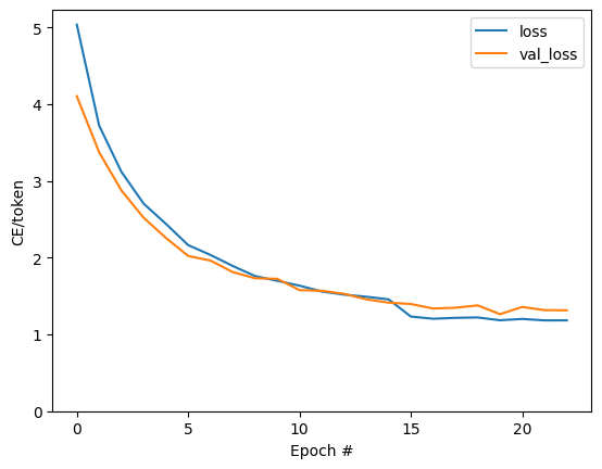
การกระโดดที่มองเห็นได้ในโครงเรื่องอยู่ที่ขอบเขตยุค
แปลภาษา
ขณะที่รูปแบบการฝึกอบรมการใช้ฟังก์ชั่นในการดำเนินการเต็มรูปแบบ text => text แปล
สำหรับวันนี้ความต้องการรูปแบบหมุนส่วน text => token IDs การทำแผนที่ให้โดย output_text_processor นอกจากนี้ยังจำเป็นต้องทราบรหัสสำหรับโทเค็นพิเศษ ทั้งหมดนี้ถูกนำมาใช้ในตัวสร้างสำหรับคลาสใหม่ การดำเนินการตามวิธีการแปลจริงจะตามมา
โดยรวมแล้วสิ่งนี้คล้ายกับการวนรอบการฝึก ยกเว้นว่าอินพุตไปยังตัวถอดรหัสในแต่ละขั้นตอนของเวลาคือตัวอย่างจากการทำนายครั้งสุดท้ายของตัวถอดรหัส
class Translator(tf.Module):

  def __init__(self, encoder, decoder, input_text_processor,
               output_text_processor):
    self.encoder = encoder
    self.decoder = decoder
    self.input_text_processor = input_text_processor
    self.output_text_processor = output_text_processor

    self.output_token_string_from_index = (
        tf.keras.layers.StringLookup(
            vocabulary=output_text_processor.get_vocabulary(),
            mask_token='',
            invert=True))

    # The output should never generate padding, unknown, or start.
    index_from_string = tf.keras.layers.StringLookup(
        vocabulary=output_text_processor.get_vocabulary(), mask_token='')
    token_mask_ids = index_from_string(['', '[UNK]', '[START]']).numpy()

    token_mask = np.zeros([index_from_string.vocabulary_size()], dtype=np.bool)
    token_mask[np.array(token_mask_ids)] = True
    self.token_mask = token_mask

    self.start_token = index_from_string(tf.constant('[START]'))
    self.end_token = index_from_string(tf.constant('[END]'))
translator = Translator(
    encoder=train_translator.encoder,
    decoder=train_translator.decoder,
    input_text_processor=input_text_processor,
    output_text_processor=output_text_processor,
)
/tmpfs/src/tf_docs_env/lib/python3.7/site-packages/ipykernel_launcher.py:21: DeprecationWarning: `np.bool` is a deprecated alias for the builtin `bool`. To silence this warning, use `bool` by itself. Doing this will not modify any behavior and is safe. If you specifically wanted the numpy scalar type, use `np.bool_` here.
Deprecated in NumPy 1.20; for more details and guidance: https://numpy.org/devdocs/release/1.20.0-notes.html#deprecations
แปลงรหัสโทเค็นเป็นข้อความ
วิธีแรกที่จะใช้เป็น tokens_to_text ซึ่งจะแปลงจากรหัสโทเค็นกับข้อความการอ่านของมนุษย์
def tokens_to_text(self, result_tokens):
  shape_checker = ShapeChecker()
  shape_checker(result_tokens, ('batch', 't'))
  result_text_tokens = self.output_token_string_from_index(result_tokens)
  shape_checker(result_text_tokens, ('batch', 't'))

  result_text = tf.strings.reduce_join(result_text_tokens,
                                       axis=1, separator=' ')
  shape_checker(result_text, ('batch'))

  result_text = tf.strings.strip(result_text)
  shape_checker(result_text, ('batch',))
  return result_text
Translator.tokens_to_text = tokens_to_text
ป้อนรหัสโทเค็นแบบสุ่มและดูว่าสร้างอะไร:
example_output_tokens = tf.random.uniform(
    shape=[5, 2], minval=0, dtype=tf.int64,
    maxval=output_text_processor.vocabulary_size())
translator.tokens_to_text(example_output_tokens).numpy()
array([b'vain mysteries', b'funny ham', b'drivers responding',
       b'mysterious ignoring', b'fashion votes'], dtype=object)
ตัวอย่างจากการทำนายของตัวถอดรหัส
ฟังก์ชันนี้ใช้เอาต์พุตบันทึกของตัวถอดรหัสและรหัสโทเค็นตัวอย่างจากการแจกจ่ายนั้น:
def sample(self, logits, temperature):
  shape_checker = ShapeChecker()
  # 't' is usually 1 here.
  shape_checker(logits, ('batch', 't', 'vocab'))
  shape_checker(self.token_mask, ('vocab',))

  token_mask = self.token_mask[tf.newaxis, tf.newaxis, :]
  shape_checker(token_mask, ('batch', 't', 'vocab'), broadcast=True)

  # Set the logits for all masked tokens to -inf, so they are never chosen.
  logits = tf.where(self.token_mask, -np.inf, logits)

  if temperature == 0.0:
    new_tokens = tf.argmax(logits, axis=-1)
  else:
    logits = tf.squeeze(logits, axis=1)
    new_tokens = tf.random.categorical(logits/temperature,
                                        num_samples=1)

  shape_checker(new_tokens, ('batch', 't'))

  return new_tokens
Translator.sample = sample
ทดสอบเรียกใช้ฟังก์ชันนี้กับอินพุตสุ่มบางตัว:
example_logits = tf.random.normal([5, 1, output_text_processor.vocabulary_size()])
example_output_tokens = translator.sample(example_logits, temperature=1.0)
example_output_tokens
<tf.Tensor: shape=(5, 1), dtype=int64, numpy=
array([[4506],
       [3577],
       [2961],
       [4586],
       [ 944]])>
ใช้ลูปการแปล
นี่คือการใช้งานลูปการแปลข้อความเป็นข้อความโดยสมบูรณ์
การดำเนินการนี้จะเก็บรวบรวมผลเป็นรายการหลามก่อนที่จะใช้ tf.concat ร่วมกับพวกเขาเข้าไปในเทนเซอร์
การดำเนินงานนี้คงหนึบกราฟออกไป max_length ซ้ำ สิ่งนี้ใช้ได้กับการดำเนินการอย่างกระตือรือร้นใน python
def translate_unrolled(self,
                       input_text, *,
                       max_length=50,
                       return_attention=True,
                       temperature=1.0):
  batch_size = tf.shape(input_text)[0]
  input_tokens = self.input_text_processor(input_text)
  enc_output, enc_state = self.encoder(input_tokens)

  dec_state = enc_state
  new_tokens = tf.fill([batch_size, 1], self.start_token)

  result_tokens = []
  attention = []
  done = tf.zeros([batch_size, 1], dtype=tf.bool)

  for _ in range(max_length):
    dec_input = DecoderInput(new_tokens=new_tokens,
                             enc_output=enc_output,
                             mask=(input_tokens!=0))

    dec_result, dec_state = self.decoder(dec_input, state=dec_state)

    attention.append(dec_result.attention_weights)

    new_tokens = self.sample(dec_result.logits, temperature)

    # If a sequence produces an `end_token`, set it `done`
    done = done | (new_tokens == self.end_token)
    # Once a sequence is done it only produces 0-padding.
    new_tokens = tf.where(done, tf.constant(0, dtype=tf.int64), new_tokens)

    # Collect the generated tokens
    result_tokens.append(new_tokens)

    if tf.executing_eagerly() and tf.reduce_all(done):
      break

  # Convert the list of generates token ids to a list of strings.
  result_tokens = tf.concat(result_tokens, axis=-1)
  result_text = self.tokens_to_text(result_tokens)

  if return_attention:
    attention_stack = tf.concat(attention, axis=1)
    return {'text': result_text, 'attention': attention_stack}
  else:
    return {'text': result_text}
Translator.translate = translate_unrolled
เรียกใช้ด้วยอินพุตง่ายๆ:
%%time
input_text = tf.constant([
    'hace mucho frio aqui.', # "It's really cold here."
    'Esta es mi vida.', # "This is my life.""
])

result = translator.translate(
    input_text = input_text)

print(result['text'][0].numpy().decode())
print(result['text'][1].numpy().decode())
print()
its a long cold here .
this is my life .

CPU times: user 165 ms, sys: 4.37 ms, total: 169 ms
Wall time: 164 ms
หากคุณต้องการที่จะส่งออกรูปแบบนี้คุณจะต้องห่อวิธีการนี้ใน tf.function การใช้งานพื้นฐานนี้มีปัญหาเล็กน้อยหากคุณพยายามทำดังนี้:
- กราฟผลลัพธ์มีขนาดใหญ่มาก และใช้เวลาสองสามวินาทีในการสร้าง บันทึก หรือโหลด
- คุณไม่สามารถทำลายจากวงคลี่แบบคงที่ดังนั้นจึงมักจะทำงาน
max_lengthซ้ำแม้ว่าผลทั้งหมดที่มีการทำ แต่ถึงอย่างนั้นมันก็เร็วกว่าการดำเนินการอย่างกระตือรือร้นเล็กน้อย
@tf.function(input_signature=[tf.TensorSpec(dtype=tf.string, shape=[None])])
def tf_translate(self, input_text):
  return self.translate(input_text)

Translator.tf_translate = tf_translate
เรียกใช้ tf.function ครั้งเพื่อรวบรวมมัน:
%%time
result = translator.tf_translate(
    input_text = input_text)
CPU times: user 18.8 s, sys: 0 ns, total: 18.8 s
Wall time: 18.7 s
%%time
result = translator.tf_translate(
    input_text = input_text)

print(result['text'][0].numpy().decode())
print(result['text'][1].numpy().decode())
print()
its very cold here .
this is my life .

CPU times: user 175 ms, sys: 0 ns, total: 175 ms
Wall time: 88 ms
[ไม่บังคับ] ใช้วงสัญลักษณ์
def translate_symbolic(self,
                       input_text,
                       *,
                       max_length=50,
                       return_attention=True,
                       temperature=1.0):
  shape_checker = ShapeChecker()
  shape_checker(input_text, ('batch',))

  batch_size = tf.shape(input_text)[0]

  # Encode the input
  input_tokens = self.input_text_processor(input_text)
  shape_checker(input_tokens, ('batch', 's'))

  enc_output, enc_state = self.encoder(input_tokens)
  shape_checker(enc_output, ('batch', 's', 'enc_units'))
  shape_checker(enc_state, ('batch', 'enc_units'))

  # Initialize the decoder
  dec_state = enc_state
  new_tokens = tf.fill([batch_size, 1], self.start_token)
  shape_checker(new_tokens, ('batch', 't1'))

  # Initialize the accumulators
  result_tokens = tf.TensorArray(tf.int64, size=1, dynamic_size=True)
  attention = tf.TensorArray(tf.float32, size=1, dynamic_size=True)
  done = tf.zeros([batch_size, 1], dtype=tf.bool)
  shape_checker(done, ('batch', 't1'))

  for t in tf.range(max_length):
    dec_input = DecoderInput(
        new_tokens=new_tokens, enc_output=enc_output, mask=(input_tokens != 0))

    dec_result, dec_state = self.decoder(dec_input, state=dec_state)

    shape_checker(dec_result.attention_weights, ('batch', 't1', 's'))
    attention = attention.write(t, dec_result.attention_weights)

    new_tokens = self.sample(dec_result.logits, temperature)
    shape_checker(dec_result.logits, ('batch', 't1', 'vocab'))
    shape_checker(new_tokens, ('batch', 't1'))

    # If a sequence produces an `end_token`, set it `done`
    done = done | (new_tokens == self.end_token)
    # Once a sequence is done it only produces 0-padding.
    new_tokens = tf.where(done, tf.constant(0, dtype=tf.int64), new_tokens)

    # Collect the generated tokens
    result_tokens = result_tokens.write(t, new_tokens)

    if tf.reduce_all(done):
      break

  # Convert the list of generated token ids to a list of strings.
  result_tokens = result_tokens.stack()
  shape_checker(result_tokens, ('t', 'batch', 't0'))
  result_tokens = tf.squeeze(result_tokens, -1)
  result_tokens = tf.transpose(result_tokens, [1, 0])
  shape_checker(result_tokens, ('batch', 't'))

  result_text = self.tokens_to_text(result_tokens)
  shape_checker(result_text, ('batch',))

  if return_attention:
    attention_stack = attention.stack()
    shape_checker(attention_stack, ('t', 'batch', 't1', 's'))

    attention_stack = tf.squeeze(attention_stack, 2)
    shape_checker(attention_stack, ('t', 'batch', 's'))

    attention_stack = tf.transpose(attention_stack, [1, 0, 2])
    shape_checker(attention_stack, ('batch', 't', 's'))

    return {'text': result_text, 'attention': attention_stack}
  else:
    return {'text': result_text}
Translator.translate = translate_symbolic
การใช้งานเริ่มต้นใช้รายการหลามเพื่อรวบรวมผลลัพธ์ การใช้งานนี้ tf.range เป็น iterator ห่วงที่ช่วยให้ tf.autograph การแปลงห่วง การเปลี่ยนแปลงที่ยิ่งใหญ่ที่สุดในการดำเนินการนี้คือการใช้ tf.TensorArray แทนหลาม list เพื่อสะสมเทนเซอร์ tf.TensorArray เป็นสิ่งจำเป็นในการเก็บรวบรวมจำนวนตัวแปรของเทนเซอร์ในโหมดกราฟ
ด้วยการดำเนินการอย่างกระตือรือร้น การใช้งานนี้มีประสิทธิภาพเทียบเท่ากับต้นฉบับ:
%%time
result = translator.translate(
    input_text = input_text)

print(result['text'][0].numpy().decode())
print(result['text'][1].numpy().decode())
print()
its very cold here .
this is my life .

CPU times: user 175 ms, sys: 0 ns, total: 175 ms
Wall time: 170 ms
แต่เมื่อคุณห่อไว้ใน tf.function คุณจะสังเกตเห็นความแตกต่างสอง
@tf.function(input_signature=[tf.TensorSpec(dtype=tf.string, shape=[None])])
def tf_translate(self, input_text):
  return self.translate(input_text)

Translator.tf_translate = tf_translate
แม่: การสร้างกราฟได้เร็วขึ้นมาก (~ 10 เท่า) เพราะมันไม่ได้สร้าง max_iterations สำเนาของรูปแบบ
%%time
result = translator.tf_translate(
    input_text = input_text)
CPU times: user 1.79 s, sys: 0 ns, total: 1.79 s
Wall time: 1.77 s
ประการที่สอง: ฟังก์ชันที่คอมไพล์เร็วกว่ามากสำหรับอินพุตขนาดเล็ก (5x ในตัวอย่างนี้) เนื่องจากสามารถแยกออกจากลูปได้
%%time
result = translator.tf_translate(
    input_text = input_text)

print(result['text'][0].numpy().decode())
print(result['text'][1].numpy().decode())
print()
its very cold here .
this is my life .

CPU times: user 40.1 ms, sys: 0 ns, total: 40.1 ms
Wall time: 17.1 ms
เห็นภาพกระบวนการ
น้ำหนักความสนใจส่งกลับโดย translate วิธีการแสดงที่รูปแบบคือ "มอง" เมื่อมันสร้างขึ้นในแต่ละโทเค็นเอาท์พุท
ดังนั้นผลรวมของความสนใจเหนือข้อมูลที่ป้อนควรส่งคืนทั้งหมด:
a = result['attention'][0]

print(np.sum(a, axis=-1))
[1.0000001 0.99999994 1. 0.99999994 1. 0.99999994]
นี่คือการแจกแจงความสนใจสำหรับขั้นตอนเอาต์พุตแรกของตัวอย่างแรก สังเกตว่าตอนนี้ความสนใจนั้นเน้นมากกว่าที่เป็นสำหรับโมเดลที่ไม่ได้รับการฝึกฝนมากเพียงใด:
_ = plt.bar(range(len(a[0, :])), a[0, :])

เนื่องจากมีการจัดตำแหน่งคร่าวๆ ระหว่างคำอินพุตและเอาต์พุต คุณจึงคาดว่าความสนใจจะโฟกัสใกล้แนวทแยง:
plt.imshow(np.array(a), vmin=0.0)
<matplotlib.image.AxesImage at 0x7faf2886ced0>

นี่คือรหัสบางส่วนเพื่อสร้างพล็อตความสนใจที่ดีขึ้น:
ป้ายกำกับ: แผนความสนใจ
def plot_attention(attention, sentence, predicted_sentence):
  sentence = tf_lower_and_split_punct(sentence).numpy().decode().split()
  predicted_sentence = predicted_sentence.numpy().decode().split() + ['[END]']
  fig = plt.figure(figsize=(10, 10))
  ax = fig.add_subplot(1, 1, 1)

  attention = attention[:len(predicted_sentence), :len(sentence)]

  ax.matshow(attention, cmap='viridis', vmin=0.0)

  fontdict = {'fontsize': 14}

  ax.set_xticklabels([''] + sentence, fontdict=fontdict, rotation=90)
  ax.set_yticklabels([''] + predicted_sentence, fontdict=fontdict)

  ax.xaxis.set_major_locator(ticker.MultipleLocator(1))
  ax.yaxis.set_major_locator(ticker.MultipleLocator(1))

  ax.set_xlabel('Input text')
  ax.set_ylabel('Output text')
  plt.suptitle('Attention weights')
i=0
plot_attention(result['attention'][i], input_text[i], result['text'][i])
/tmpfs/src/tf_docs_env/lib/python3.7/site-packages/ipykernel_launcher.py:14: UserWarning: FixedFormatter should only be used together with FixedLocator

/tmpfs/src/tf_docs_env/lib/python3.7/site-packages/ipykernel_launcher.py:15: UserWarning: FixedFormatter should only be used together with FixedLocator
  from ipykernel import kernelapp as app
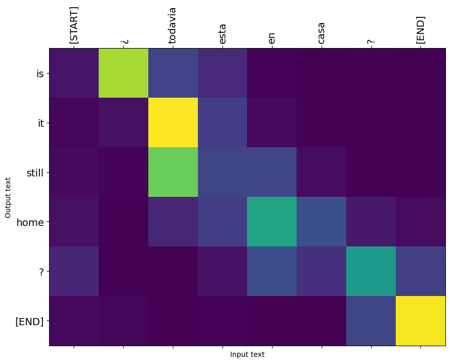
แปลประโยคอีกสองสามประโยคและวางแผน:
%%time
three_input_text = tf.constant([
    # This is my life.
    'Esta es mi vida.',
    # Are they still home?
    '¿Todavía están en casa?',
    # Try to find out.'
    'Tratar de descubrir.',
])

result = translator.tf_translate(three_input_text)

for tr in result['text']:
  print(tr.numpy().decode())

print()
this is my life .
are you still at home ?
all about killed .

CPU times: user 78 ms, sys: 23 ms, total: 101 ms
Wall time: 23.1 ms
result['text']
<tf.Tensor: shape=(3,), dtype=string, numpy=
array([b'this is my life .', b'are you still at home ?',
       b'all about killed .'], dtype=object)>
i = 0
plot_attention(result['attention'][i], three_input_text[i], result['text'][i])
/tmpfs/src/tf_docs_env/lib/python3.7/site-packages/ipykernel_launcher.py:14: UserWarning: FixedFormatter should only be used together with FixedLocator

/tmpfs/src/tf_docs_env/lib/python3.7/site-packages/ipykernel_launcher.py:15: UserWarning: FixedFormatter should only be used together with FixedLocator
  from ipykernel import kernelapp as app

i = 1
plot_attention(result['attention'][i], three_input_text[i], result['text'][i])
/tmpfs/src/tf_docs_env/lib/python3.7/site-packages/ipykernel_launcher.py:14: UserWarning: FixedFormatter should only be used together with FixedLocator

/tmpfs/src/tf_docs_env/lib/python3.7/site-packages/ipykernel_launcher.py:15: UserWarning: FixedFormatter should only be used together with FixedLocator
  from ipykernel import kernelapp as app

i = 2
plot_attention(result['attention'][i], three_input_text[i], result['text'][i])
/tmpfs/src/tf_docs_env/lib/python3.7/site-packages/ipykernel_launcher.py:14: UserWarning: FixedFormatter should only be used together with FixedLocator

/tmpfs/src/tf_docs_env/lib/python3.7/site-packages/ipykernel_launcher.py:15: UserWarning: FixedFormatter should only be used together with FixedLocator
  from ipykernel import kernelapp as app

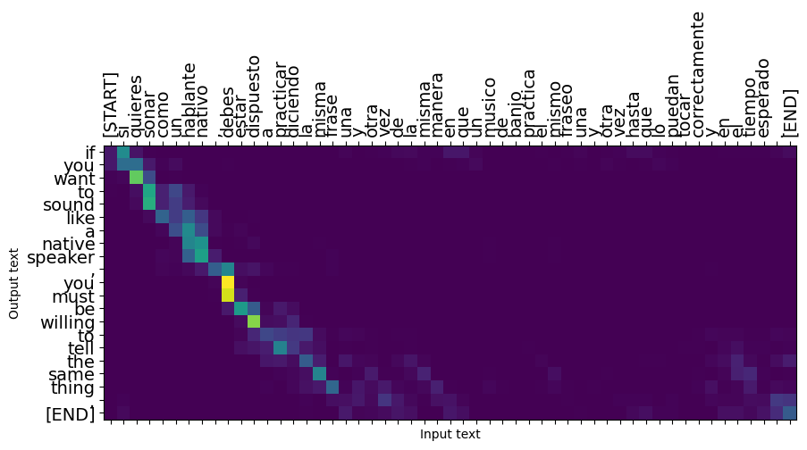
ประโยคสั้นๆ มักจะใช้ได้ผลดี แต่ถ้าอินพุตยาวเกินไป โมเดลจะสูญเสียโฟกัสไปและหยุดให้การคาดการณ์ที่สมเหตุสมผล มีสองสาเหตุหลักสำหรับสิ่งนี้:
- โมเดลนี้ได้รับการฝึกฝนโดยครูบังคับให้ป้อนโทเค็นที่ถูกต้องในแต่ละขั้นตอน โดยไม่คำนึงถึงการคาดการณ์ของโมเดล แบบจำลองนี้สามารถทำให้แข็งแกร่งขึ้นได้หากบางครั้งได้รับการคาดการณ์ด้วยตัวมันเอง
- โมเดลมีสิทธิ์เข้าถึงเอาต์พุตก่อนหน้าผ่านสถานะ RNN เท่านั้น หากสถานะ RNN เสียหาย จะไม่มีทางที่แบบจำลองจะกู้คืนได้ หม้อแปลง แก้ปัญหานี้โดยใช้ความสนใจของตัวเองในการเข้ารหัสและถอดรหัส
long_input_text = tf.constant([inp[-1]])

import textwrap
print('Expected output:\n', '\n'.join(textwrap.wrap(targ[-1])))
Expected output:
 If you want to sound like a native speaker, you must be willing to
practice saying the same sentence over and over in the same way that
banjo players practice the same phrase over and over until they can
play it correctly and at the desired tempo.
result = translator.tf_translate(long_input_text)

i = 0
plot_attention(result['attention'][i], long_input_text[i], result['text'][i])
_ = plt.suptitle('This never works')
/tmpfs/src/tf_docs_env/lib/python3.7/site-packages/ipykernel_launcher.py:14: UserWarning: FixedFormatter should only be used together with FixedLocator

/tmpfs/src/tf_docs_env/lib/python3.7/site-packages/ipykernel_launcher.py:15: UserWarning: FixedFormatter should only be used together with FixedLocator
  from ipykernel import kernelapp as app
ส่งออก
เมื่อคุณมีรูปแบบที่คุณพอใจกับคุณอาจต้องการที่จะส่งออกเป็น tf.saved_model สำหรับใช้ภายนอกของโปรแกรมหลามที่สร้างมันขึ้นมา
ตั้งแต่รูปแบบเป็น subclass ของ tf.Module (ผ่าน keras.Model ) และทุกฟังก์ชั่นสำหรับการส่งออกจะรวบรวมใน tf.function รูปแบบควรส่งออกหมดจดด้วย tf.saved_model.save :
ตอนนี้ฟังก์ชั่นที่ได้รับการตรวจสอบก็จะสามารถส่งออกโดยใช้ saved_model.save :
tf.saved_model.save(translator, 'translator',
                    signatures={'serving_default': translator.tf_translate})
2021-12-04 12:27:54.310890: W tensorflow/python/util/util.cc:368] Sets are not currently considered sequences, but this may change in the future, so consider avoiding using them.
WARNING:absl:Found untraced functions such as encoder_2_layer_call_fn, encoder_2_layer_call_and_return_conditional_losses, decoder_2_layer_call_fn, decoder_2_layer_call_and_return_conditional_losses, embedding_4_layer_call_fn while saving (showing 5 of 60). These functions will not be directly callable after loading.
INFO:tensorflow:Assets written to: translator/assets
INFO:tensorflow:Assets written to: translator/assets
reloaded = tf.saved_model.load('translator')
result = reloaded.tf_translate(three_input_text)
%%time
result = reloaded.tf_translate(three_input_text)

for tr in result['text']:
  print(tr.numpy().decode())

print()
this is my life .
are you still at home ?
find out about to find out .

CPU times: user 42.8 ms, sys: 7.69 ms, total: 50.5 ms
Wall time: 20 ms
ขั้นตอนถัดไป
- ดาวน์โหลดชุดข้อมูลที่แตกต่างกัน ในการทดสอบที่มีการแปล, ตัวอย่างเช่นภาษาอังกฤษเป็นภาษาเยอรมันหรือภาษาอังกฤษเป็นภาษาฝรั่งเศส
- ทดลองกับการฝึกกับชุดข้อมูลที่ใหญ่ขึ้น หรือใช้ช่วงเวลาที่มากขึ้น
- ลอง หม้อแปลงกวดวิชา ซึ่งดำเนินงานแปลที่คล้ายกัน แต่ใช้ชั้นหม้อแปลงแทน RNNs รุ่นนี้ยังใช้
text.BertTokenizerจะใช้ tokenization wordpiece - มีลักษณะที่เป็น tensorflow_addons.seq2seq สำหรับการดำเนินการจัดเรียงของลำดับนี้กับรูปแบบลำดับ
tfa.seq2seqแพคเกจรวมถึงฟังก์ชั่นระดับที่สูงขึ้นเช่นseq2seq.BeamSearchDecoder