TF-Hub CORD-19 Swivel 임베딩 살펴보기

TensorFlow.org에서 보기

Google Colab에서 실행

GitHub에서 보기

노트북 다운로드

TF Hub 모델 보기

TF-Hub(https://tfhub.dev/tensorflow/cord-19/swivel-128d/3)의 CORD-19 Swivel 텍스트 임베딩 모듈은 연구원들이 코로나바이러스감염증-19와 관련된 자연어 텍스트를 분석할 수 있도록 빌드되었습니다. 이러한 임베딩은 CORD-19 데이터세트에 있는 기사의 제목, 저자, 요약문, 본문 텍스트 및 참조 제목에 대해 훈련되었습니다.

이 colab에서는 다음을 수행합니다.

임베딩 공간에서 의미론적으로 유사한 단어를 분석합니다.
CORD-19 임베딩을 사용하여 SciCite 데이터세트에서 분류자를 훈련합니다.

설정

import functools
import itertools
import matplotlib.pyplot as plt
import numpy as np
import seaborn as sns
import pandas as pd

import tensorflow as tf

import tensorflow_datasets as tfds
import tensorflow_hub as hub

from tqdm import trange

2022-12-14 20:59:19.175950: W tensorflow/compiler/xla/stream_executor/platform/default/dso_loader.cc:64] Could not load dynamic library 'libnvinfer.so.7'; dlerror: libnvinfer.so.7: cannot open shared object file: No such file or directory
2022-12-14 20:59:19.176062: W tensorflow/compiler/xla/stream_executor/platform/default/dso_loader.cc:64] Could not load dynamic library 'libnvinfer_plugin.so.7'; dlerror: libnvinfer_plugin.so.7: cannot open shared object file: No such file or directory
2022-12-14 20:59:19.176072: W tensorflow/compiler/tf2tensorrt/utils/py_utils.cc:38] TF-TRT Warning: Cannot dlopen some TensorRT libraries. If you would like to use Nvidia GPU with TensorRT, please make sure the missing libraries mentioned above are installed properly.

임베딩 분석하기

서로 다른 용어 간의 상관 행렬을 계산하고 플롯하여 임베딩을 분석하는 것으로 시작하겠습니다. 임베딩이 여러 단어의 의미를 성공적으로 포착하는 방법을 학습한 경우, 의미론적으로 유사한 단어의 임베딩 벡터는 서로 가까워야 합니다. 코로나바이러스감염증-19와 관련된 일부 용어를 살펴보겠습니다.

# Use the inner product between two embedding vectors as the similarity measure
def plot_correlation(labels, features):
  corr = np.inner(features, features)
  corr /= np.max(corr)
  sns.heatmap(corr, xticklabels=labels, yticklabels=labels)

# Generate embeddings for some terms
queries = [
  # Related viruses
  'coronavirus', 'SARS', 'MERS',
  # Regions
  'Italy', 'Spain', 'Europe',
  # Symptoms
  'cough', 'fever', 'throat'
]

module = hub.load('https://tfhub.dev/tensorflow/cord-19/swivel-128d/3')
embeddings = module(queries)

plot_correlation(queries, embeddings)

png

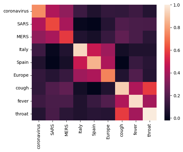
임베딩이 여러 용어의 의미를 성공적으로 포착했음을 알 수 있습니다. 각 단어는 해당 클러스터의 다른 단어와 유사하지만(즉, "coronavirus"는 "SARS" 및 "MERS"와 높은 상관 관계가 있음) 다른 클러스터의 용어와는 다릅니다(즉, "SARS"와 "Spain" 사이의 유사성은 0에 가까움).

이제 이러한 임베딩을 사용하여 특정 작업을 해결하는 방법을 살펴보겠습니다.

SciCite: 인용 의도 분류

이 섹션에서는 텍스트 분류와 같은 다운스트림 작업에 임베딩을 사용하는 방법을 보여줍니다. TensorFlow 데이터세트의 SciCite 데이터세트를 사용하여 학술 논문에서 인용 의도를 분류합니다. 학술 논문의 인용이 포함된 문장이 주어지면 인용의 주요 의도가 배경 정보, 방법 사용 또는 결과 비교인지 여부를 분류합니다.

builder = tfds.builder(name='scicite')
builder.download_and_prepare()
train_data, validation_data, test_data = builder.as_dataset(
    split=('train', 'validation', 'test'),
    as_supervised=True)

Let's take a look at a few labeled examples from the training set

NUM_EXAMPLES =   10

TEXT_FEATURE_NAME = builder.info.supervised_keys[0]
LABEL_NAME = builder.info.supervised_keys[1]

def label2str(numeric_label):
  m = builder.info.features[LABEL_NAME].names
  return m[numeric_label]

data = next(iter(train_data.batch(NUM_EXAMPLES)))


pd.DataFrame({
    TEXT_FEATURE_NAME: [ex.numpy().decode('utf8') for ex in data[0]],
    LABEL_NAME: [label2str(x) for x in data[1]]
})

인용 의도 분류자 훈련하기

Keras를 사용하여 SciCite 데이터세트에 대한 분류자를 훈련합니다. 분류 레이어를 상위에 둔 CORD-19 임베딩을 사용하는 모델을 빌드하겠습니다.

Hyperparameters

EMBEDDING = 'https://tfhub.dev/tensorflow/cord-19/swivel-128d/3' 
TRAINABLE_MODULE = False 

hub_layer = hub.KerasLayer(EMBEDDING, input_shape=[], 
                           dtype=tf.string, trainable=TRAINABLE_MODULE)

model = tf.keras.Sequential()
model.add(hub_layer)
model.add(tf.keras.layers.Dense(3))
model.summary()
model.compile(optimizer='adam',
              loss=tf.keras.losses.SparseCategoricalCrossentropy(from_logits=True),
              metrics=['accuracy'])

WARNING:tensorflow:Please fix your imports. Module tensorflow.python.training.tracking.data_structures has been moved to tensorflow.python.trackable.data_structures. The old module will be deleted in version 2.11.
WARNING:tensorflow:Please fix your imports. Module tensorflow.python.training.tracking.data_structures has been moved to tensorflow.python.trackable.data_structures. The old module will be deleted in version 2.11.
WARNING:tensorflow:From /tmpfs/src/tf_docs_env/lib/python3.9/site-packages/tensorflow/python/autograph/pyct/static_analysis/liveness.py:83: Analyzer.lamba_check (from tensorflow.python.autograph.pyct.static_analysis.liveness) is deprecated and will be removed after 2023-09-23.
Instructions for updating:
Lambda fuctions will be no more assumed to be used in the statement where they are used, or at least in the same block. https://github.com/tensorflow/tensorflow/issues/56089
WARNING:tensorflow:From /tmpfs/src/tf_docs_env/lib/python3.9/site-packages/tensorflow/python/autograph/pyct/static_analysis/liveness.py:83: Analyzer.lamba_check (from tensorflow.python.autograph.pyct.static_analysis.liveness) is deprecated and will be removed after 2023-09-23.
Instructions for updating:
Lambda fuctions will be no more assumed to be used in the statement where they are used, or at least in the same block. https://github.com/tensorflow/tensorflow/issues/56089
Model: "sequential"
_________________________________________________________________
 Layer (type)                Output Shape              Param #   
=================================================================
 keras_layer (KerasLayer)    (None, 128)               17301632  
                                                                 
 dense (Dense)               (None, 3)                 387       
                                                                 
=================================================================
Total params: 17,302,019
Trainable params: 387
Non-trainable params: 17,301,632
_________________________________________________________________

모델 훈련 및 평가하기

SciCite 작업의 성능을 확인하기 위해 모델을 훈련하고 평가하겠습니다.

EPOCHS = 35
BATCH_SIZE = 32

history = model.fit(train_data.shuffle(10000).batch(BATCH_SIZE),
                    epochs=EPOCHS,
                    validation_data=validation_data.batch(BATCH_SIZE),
                    verbose=1)

Epoch 1/35
257/257 [==============================] - 3s 5ms/step - loss: 0.8662 - accuracy: 0.6333 - val_loss: 0.7538 - val_accuracy: 0.6932
Epoch 2/35
257/257 [==============================] - 1s 4ms/step - loss: 0.6827 - accuracy: 0.7269 - val_loss: 0.6606 - val_accuracy: 0.7555
Epoch 3/35
257/257 [==============================] - 1s 4ms/step - loss: 0.6159 - accuracy: 0.7617 - val_loss: 0.6189 - val_accuracy: 0.7598
Epoch 4/35
257/257 [==============================] - 1s 4ms/step - loss: 0.5836 - accuracy: 0.7711 - val_loss: 0.5991 - val_accuracy: 0.7697
Epoch 5/35
257/257 [==============================] - 1s 5ms/step - loss: 0.5653 - accuracy: 0.7801 - val_loss: 0.5868 - val_accuracy: 0.7664
Epoch 6/35
257/257 [==============================] - 1s 4ms/step - loss: 0.5535 - accuracy: 0.7841 - val_loss: 0.5771 - val_accuracy: 0.7686
Epoch 7/35
257/257 [==============================] - 1s 4ms/step - loss: 0.5449 - accuracy: 0.7884 - val_loss: 0.5719 - val_accuracy: 0.7729
Epoch 8/35
257/257 [==============================] - 1s 4ms/step - loss: 0.5385 - accuracy: 0.7913 - val_loss: 0.5677 - val_accuracy: 0.7751
Epoch 9/35
257/257 [==============================] - 1s 4ms/step - loss: 0.5335 - accuracy: 0.7919 - val_loss: 0.5627 - val_accuracy: 0.7729
Epoch 10/35
257/257 [==============================] - 1s 4ms/step - loss: 0.5285 - accuracy: 0.7940 - val_loss: 0.5611 - val_accuracy: 0.7707
Epoch 11/35
257/257 [==============================] - 1s 4ms/step - loss: 0.5253 - accuracy: 0.7958 - val_loss: 0.5574 - val_accuracy: 0.7751
Epoch 12/35
257/257 [==============================] - 2s 5ms/step - loss: 0.5222 - accuracy: 0.7933 - val_loss: 0.5539 - val_accuracy: 0.7751
Epoch 13/35
257/257 [==============================] - 1s 4ms/step - loss: 0.5201 - accuracy: 0.7941 - val_loss: 0.5523 - val_accuracy: 0.7762
Epoch 14/35
257/257 [==============================] - 1s 4ms/step - loss: 0.5179 - accuracy: 0.7951 - val_loss: 0.5518 - val_accuracy: 0.7762
Epoch 15/35
257/257 [==============================] - 2s 5ms/step - loss: 0.5154 - accuracy: 0.7959 - val_loss: 0.5496 - val_accuracy: 0.7795
Epoch 16/35
257/257 [==============================] - 1s 4ms/step - loss: 0.5138 - accuracy: 0.7975 - val_loss: 0.5517 - val_accuracy: 0.7784
Epoch 17/35
257/257 [==============================] - 2s 4ms/step - loss: 0.5119 - accuracy: 0.7977 - val_loss: 0.5549 - val_accuracy: 0.7751
Epoch 18/35
257/257 [==============================] - 1s 4ms/step - loss: 0.5114 - accuracy: 0.7979 - val_loss: 0.5473 - val_accuracy: 0.7795
Epoch 19/35
257/257 [==============================] - 1s 4ms/step - loss: 0.5101 - accuracy: 0.7994 - val_loss: 0.5471 - val_accuracy: 0.7795
Epoch 20/35
257/257 [==============================] - 1s 4ms/step - loss: 0.5091 - accuracy: 0.7974 - val_loss: 0.5488 - val_accuracy: 0.7784
Epoch 21/35
257/257 [==============================] - 2s 5ms/step - loss: 0.5070 - accuracy: 0.8000 - val_loss: 0.5491 - val_accuracy: 0.7806
Epoch 22/35
257/257 [==============================] - 2s 5ms/step - loss: 0.5068 - accuracy: 0.8011 - val_loss: 0.5451 - val_accuracy: 0.7838
Epoch 23/35
257/257 [==============================] - 1s 5ms/step - loss: 0.5057 - accuracy: 0.8002 - val_loss: 0.5482 - val_accuracy: 0.7817
Epoch 24/35
257/257 [==============================] - 1s 4ms/step - loss: 0.5049 - accuracy: 0.8003 - val_loss: 0.5477 - val_accuracy: 0.7806
Epoch 25/35
257/257 [==============================] - 1s 4ms/step - loss: 0.5042 - accuracy: 0.8007 - val_loss: 0.5474 - val_accuracy: 0.7828
Epoch 26/35
257/257 [==============================] - 1s 4ms/step - loss: 0.5035 - accuracy: 0.7999 - val_loss: 0.5453 - val_accuracy: 0.7860
Epoch 27/35
257/257 [==============================] - 1s 4ms/step - loss: 0.5027 - accuracy: 0.8007 - val_loss: 0.5464 - val_accuracy: 0.7871
Epoch 28/35
257/257 [==============================] - 1s 4ms/step - loss: 0.5021 - accuracy: 0.8018 - val_loss: 0.5460 - val_accuracy: 0.7882
Epoch 29/35
257/257 [==============================] - 2s 5ms/step - loss: 0.5015 - accuracy: 0.8035 - val_loss: 0.5450 - val_accuracy: 0.7871
Epoch 30/35
257/257 [==============================] - 1s 4ms/step - loss: 0.5013 - accuracy: 0.8018 - val_loss: 0.5448 - val_accuracy: 0.7849
Epoch 31/35
257/257 [==============================] - 2s 5ms/step - loss: 0.5003 - accuracy: 0.8008 - val_loss: 0.5443 - val_accuracy: 0.7871
Epoch 32/35
257/257 [==============================] - 2s 5ms/step - loss: 0.5002 - accuracy: 0.8000 - val_loss: 0.5428 - val_accuracy: 0.7882
Epoch 33/35
257/257 [==============================] - 2s 5ms/step - loss: 0.5003 - accuracy: 0.8016 - val_loss: 0.5443 - val_accuracy: 0.7849
Epoch 34/35
257/257 [==============================] - 1s 5ms/step - loss: 0.4999 - accuracy: 0.8024 - val_loss: 0.5447 - val_accuracy: 0.7871
Epoch 35/35
257/257 [==============================] - 1s 5ms/step - loss: 0.4989 - accuracy: 0.8021 - val_loss: 0.5433 - val_accuracy: 0.7893

from matplotlib import pyplot as plt
def display_training_curves(training, validation, title, subplot):
  if subplot%10==1: # set up the subplots on the first call
    plt.subplots(figsize=(10,10), facecolor='#F0F0F0')
    plt.tight_layout()
  ax = plt.subplot(subplot)
  ax.set_facecolor('#F8F8F8')
  ax.plot(training)
  ax.plot(validation)
  ax.set_title('model '+ title)
  ax.set_ylabel(title)
  ax.set_xlabel('epoch')
  ax.legend(['train', 'valid.'])

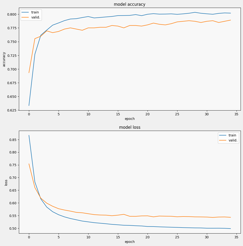
display_training_curves(history.history['accuracy'], history.history['val_accuracy'], 'accuracy', 211)
display_training_curves(history.history['loss'], history.history['val_loss'], 'loss', 212)

/tmpfs/tmp/ipykernel_59833/4094752860.py:6: MatplotlibDeprecationWarning: Auto-removal of overlapping axes is deprecated since 3.6 and will be removed two minor releases later; explicitly call ax.remove() as needed.
  ax = plt.subplot(subplot)

png

모델 평가하기

그리고 모델이 어떤 성능을 보이는지 알아보겠습니다. 손실(오류를 나타내는 숫자, 값이 낮을수록 좋음) 및 정확성의 두 가지 값이 반환됩니다.

results = model.evaluate(test_data.batch(512), verbose=2)

for name, value in zip(model.metrics_names, results):
  print('%s: %.3f' % (name, value))

4/4 - 0s - loss: 0.5347 - accuracy: 0.7907 - 265ms/epoch - 66ms/step
loss: 0.535
accuracy: 0.791

특히 정확성이 빠르게 증가하는 동안 손실이 빠르게 감소하는 것을 볼 수 있습니다. 예측이 실제 레이블과 어떻게 관련되는지 확인하기 위해 몇 가지 예를 플롯해 보겠습니다.

prediction_dataset = next(iter(test_data.batch(20)))

prediction_texts = [ex.numpy().decode('utf8') for ex in prediction_dataset[0]]
prediction_labels = [label2str(x) for x in prediction_dataset[1]]

predictions = [
    label2str(x) for x in np.argmax(model.predict(prediction_texts), axis=-1)]


pd.DataFrame({
    TEXT_FEATURE_NAME: prediction_texts,
    LABEL_NAME: prediction_labels,
    'prediction': predictions
})

1/1 [==============================] - 0s 153ms/step

이 무작위 샘플의 경우 모델이 대부분 올바른 레이블을 예측하여 과학적 문장을 상당히 잘 포함할 수 있음을 알 수 있습니다.

다음 단계

이제 TF-Hub의 CORD-19 Swivel 임베딩에 대해 조금 더 알게 되었으므로 CORD-19 Kaggle 대회에 참여하여 코로나바이러스감염증-19 관련 학술 텍스트에서 과학적 통찰력을 얻는 데 기여해 보세요.

CORD-19 Kaggle 챌린지에 참여하세요.
코로나바이러스감염증-19 공개 연구 데이터세트(CORD-19)에 대해 자세히 알아보세요.
https://tfhub.dev/tensorflow/cord-19/swivel-128d/3에서 설명서를 참조하고 TF-Hub 임베딩에 대한 자세히 알아보세요.
TensorFlow 임베딩 프로젝터로 CORD-19 임베딩 공간을 탐색해 보세요.

TF-Hub CORD-19 Swivel 임베딩 살펴보기 컬렉션을 사용해 정리하기 내 환경설정을 기준으로 콘텐츠를 저장하고 분류하세요.

설정