Buku catatan ini mengilustrasikan dua contoh pemasangan model deret waktu struktural ke deret waktu dan menggunakannya untuk menghasilkan prakiraan dan penjelasan.
| | |  Lihat sumber di GitHub Lihat sumber di GitHub | |
Dependensi & Prasyarat
Impor dan atur
%matplotlib inline
import matplotlib as mpl
from matplotlib import pylab as plt
import matplotlib.dates as mdates
import seaborn as sns

import collections

import numpy as np
import tensorflow.compat.v2 as tf
import tensorflow_probability as tfp

from tensorflow_probability import distributions as tfd
from tensorflow_probability import sts

tf.enable_v2_behavior()
Membuat hal-hal Cepat!
Sebelum kita masuk, pastikan kita menggunakan GPU untuk demo ini.
Untuk melakukan ini, pilih "Runtime" -> "Ubah jenis runtime" -> "Akselerator perangkat keras" -> "GPU".
Cuplikan berikut akan memverifikasi bahwa kami memiliki akses ke GPU.
if tf.test.gpu_device_name() != '/device:GPU:0':
  print('WARNING: GPU device not found.')
else:
  print('SUCCESS: Found GPU: {}'.format(tf.test.gpu_device_name()))
SUCCESS: Found GPU: /device:GPU:0
Pengaturan plot
Metode pembantu untuk merencanakan deret waktu dan prakiraan.
from pandas.plotting import register_matplotlib_converters
register_matplotlib_converters()

sns.set_context("notebook", font_scale=1.)
sns.set_style("whitegrid")
%config InlineBackend.figure_format = 'retina'
def plot_forecast(x, y,
                  forecast_mean, forecast_scale, forecast_samples,
                  title, x_locator=None, x_formatter=None):
  """Plot a forecast distribution against the 'true' time series."""
  colors = sns.color_palette()
  c1, c2 = colors[0], colors[1]
  fig = plt.figure(figsize=(12, 6))
  ax = fig.add_subplot(1, 1, 1)

  num_steps = len(y)
  num_steps_forecast = forecast_mean.shape[-1]
  num_steps_train = num_steps - num_steps_forecast


  ax.plot(x, y, lw=2, color=c1, label='ground truth')

  forecast_steps = np.arange(
      x[num_steps_train],
      x[num_steps_train]+num_steps_forecast,
      dtype=x.dtype)

  ax.plot(forecast_steps, forecast_samples.T, lw=1, color=c2, alpha=0.1)

  ax.plot(forecast_steps, forecast_mean, lw=2, ls='--', color=c2,
           label='forecast')
  ax.fill_between(forecast_steps,
                   forecast_mean-2*forecast_scale,
                   forecast_mean+2*forecast_scale, color=c2, alpha=0.2)

  ymin, ymax = min(np.min(forecast_samples), np.min(y)), max(np.max(forecast_samples), np.max(y))
  yrange = ymax-ymin
  ax.set_ylim([ymin - yrange*0.1, ymax + yrange*0.1])
  ax.set_title("{}".format(title))
  ax.legend()

  if x_locator is not None:
    ax.xaxis.set_major_locator(x_locator)
    ax.xaxis.set_major_formatter(x_formatter)
    fig.autofmt_xdate()

  return fig, ax
def plot_components(dates,
                    component_means_dict,
                    component_stddevs_dict,
                    x_locator=None,
                    x_formatter=None):
  """Plot the contributions of posterior components in a single figure."""
  colors = sns.color_palette()
  c1, c2 = colors[0], colors[1]

  axes_dict = collections.OrderedDict()
  num_components = len(component_means_dict)
  fig = plt.figure(figsize=(12, 2.5 * num_components))
  for i, component_name in enumerate(component_means_dict.keys()):
    component_mean = component_means_dict[component_name]
    component_stddev = component_stddevs_dict[component_name]

    ax = fig.add_subplot(num_components,1,1+i)
    ax.plot(dates, component_mean, lw=2)
    ax.fill_between(dates,
                     component_mean-2*component_stddev,
                     component_mean+2*component_stddev,
                     color=c2, alpha=0.5)
    ax.set_title(component_name)
    if x_locator is not None:
      ax.xaxis.set_major_locator(x_locator)
      ax.xaxis.set_major_formatter(x_formatter)
    axes_dict[component_name] = ax
  fig.autofmt_xdate()
  fig.tight_layout()
  return fig, axes_dict
def plot_one_step_predictive(dates, observed_time_series,
                             one_step_mean, one_step_scale,
                             x_locator=None, x_formatter=None):
  """Plot a time series against a model's one-step predictions."""

  colors = sns.color_palette()
  c1, c2 = colors[0], colors[1]

  fig=plt.figure(figsize=(12, 6))
  ax = fig.add_subplot(1,1,1)
  num_timesteps = one_step_mean.shape[-1]
  ax.plot(dates, observed_time_series, label="observed time series", color=c1)
  ax.plot(dates, one_step_mean, label="one-step prediction", color=c2)
  ax.fill_between(dates,
                  one_step_mean - one_step_scale,
                  one_step_mean + one_step_scale,
                  alpha=0.1, color=c2)
  ax.legend()

  if x_locator is not None:
    ax.xaxis.set_major_locator(x_locator)
    ax.xaxis.set_major_formatter(x_formatter)
    fig.autofmt_xdate()
  fig.tight_layout()
  return fig, ax
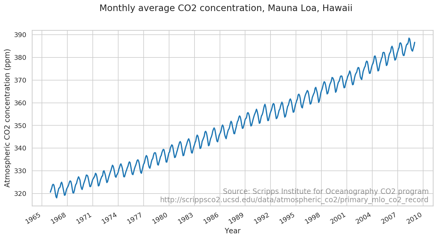
Rekor CO2 Mauna Loa
Kami akan mendemonstrasikan pemasangan model dengan pembacaan CO2 atmosfer dari observatorium Mauna Loa.
Data
# CO2 readings from Mauna Loa observatory, monthly beginning January 1966
# Original source: http://scrippsco2.ucsd.edu/data/atmospheric_co2/primary_mlo_co2_record
co2_by_month = np.array('320.62,321.60,322.39,323.70,324.08,323.75,322.38,320.36,318.64,318.10,319.78,321.03,322.33,322.50,323.04,324.42,325.00,324.09,322.54,320.92,319.25,319.39,320.73,321.96,322.57,323.15,323.89,325.02,325.57,325.36,324.14,322.11,320.33,320.25,321.32,322.89,324.00,324.42,325.63,326.66,327.38,326.71,325.88,323.66,322.38,321.78,322.85,324.12,325.06,325.98,326.93,328.14,328.08,327.67,326.34,324.69,323.10,323.06,324.01,325.13,326.17,326.68,327.17,327.79,328.92,328.57,327.36,325.43,323.36,323.56,324.80,326.01,326.77,327.63,327.75,329.73,330.07,329.09,328.04,326.32,324.84,325.20,326.50,327.55,328.55,329.56,330.30,331.50,332.48,332.07,330.87,329.31,327.51,327.18,328.16,328.64,329.35,330.71,331.48,332.65,333.09,332.25,331.18,329.39,327.43,327.37,328.46,329.57,330.40,331.40,332.04,333.31,333.97,333.60,331.90,330.06,328.56,328.34,329.49,330.76,331.75,332.56,333.50,334.58,334.88,334.33,333.05,330.94,329.30,328.94,330.31,331.68,332.93,333.42,334.70,336.07,336.75,336.27,334.92,332.75,331.59,331.16,332.40,333.85,334.97,335.38,336.64,337.76,338.01,337.89,336.54,334.68,332.76,332.55,333.92,334.95,336.23,336.76,337.96,338.88,339.47,339.29,337.73,336.09,333.92,333.86,335.29,336.73,338.01,338.36,340.07,340.77,341.47,341.17,339.56,337.60,335.88,336.02,337.10,338.21,339.24,340.48,341.38,342.51,342.91,342.25,340.49,338.43,336.69,336.86,338.36,339.61,340.75,341.61,342.70,343.57,344.14,343.35,342.06,339.81,337.98,337.86,339.26,340.49,341.38,342.52,343.10,344.94,345.76,345.32,343.98,342.38,339.87,339.99,341.15,342.99,343.70,344.50,345.28,347.06,347.43,346.80,345.39,343.28,341.07,341.35,342.98,344.22,344.97,345.99,347.42,348.35,348.93,348.25,346.56,344.67,343.09,342.80,344.24,345.56,346.30,346.95,347.85,349.55,350.21,349.55,347.94,345.90,344.85,344.17,345.66,346.90,348.02,348.48,349.42,350.99,351.85,351.26,349.51,348.10,346.45,346.36,347.81,348.96,350.43,351.73,352.22,353.59,354.22,353.79,352.38,350.43,348.73,348.88,350.07,351.34,352.76,353.07,353.68,355.42,355.67,355.12,353.90,351.67,349.80,349.99,351.30,352.52,353.66,354.70,355.38,356.20,357.16,356.23,354.81,352.91,350.96,351.18,352.83,354.21,354.72,355.75,357.16,358.60,359.34,358.24,356.17,354.02,352.15,352.21,353.75,354.99,355.99,356.72,357.81,359.15,359.66,359.25,357.02,355.00,353.01,353.31,354.16,355.40,356.70,357.17,358.38,359.46,360.28,359.60,357.57,355.52,353.69,353.99,355.34,356.80,358.37,358.91,359.97,361.26,361.69,360.94,359.55,357.48,355.84,356.00,357.58,359.04,359.97,361.00,361.64,363.45,363.80,363.26,361.89,359.45,358.05,357.75,359.56,360.70,362.05,363.24,364.02,364.71,365.41,364.97,363.65,361.48,359.45,359.61,360.76,362.33,363.18,363.99,364.56,366.36,366.80,365.63,364.47,362.50,360.19,360.78,362.43,364.28,365.33,366.15,367.31,368.61,369.30,368.88,367.64,365.78,363.90,364.23,365.46,366.97,368.15,368.87,369.59,371.14,371.00,370.35,369.27,366.93,364.64,365.13,366.68,368.00,369.14,369.46,370.51,371.66,371.83,371.69,370.12,368.12,366.62,366.73,368.29,369.53,370.28,371.50,372.12,372.86,374.02,373.31,371.62,369.55,367.96,368.09,369.68,371.24,372.44,373.08,373.52,374.85,375.55,375.40,374.02,371.48,370.70,370.25,372.08,373.78,374.68,375.62,376.11,377.65,378.35,378.13,376.61,374.48,372.98,373.00,374.35,375.69,376.79,377.36,378.39,380.50,380.62,379.55,377.76,375.83,374.05,374.22,375.84,377.44,378.34,379.61,380.08,382.05,382.24,382.08,380.67,378.67,376.42,376.80,378.31,379.96,381.37,382.02,382.56,384.37,384.92,384.03,382.28,380.48,378.81,379.06,380.14,381.66,382.58,383.71,384.34,386.23,386.41,385.87,384.45,381.84,380.86,380.86,382.36,383.61,385.07,385.84,385.83,386.77,388.51,388.05,386.25,384.08,383.09,382.78,384.01,385.11,386.65,387.12,388.52,389.57,390.16,389.62,388.07,386.08,384.65,384.33,386.05,387.49,388.55,390.07,391.01,392.38,393.22,392.24,390.33,388.52,386.84,387.16,388.67,389.81,391.30,391.92,392.45,393.37,394.28,393.69,392.59,390.21,389.00,388.93,390.24,391.80,393.07,393.35,394.36,396.43,396.87,395.88,394.52,392.54,391.13,391.01,392.95,394.34,395.61,396.85,397.26,398.35,399.98,398.87,397.37,395.41,393.39,393.70,395.19,396.82,397.92,398.10,399.47,401.33,401.88,401.31,399.07,397.21,395.40,395.65,397.23,398.79,399.85,400.31,401.51,403.45,404.10,402.88,401.61,399.00,397.50,398.28,400.24,401.89,402.65,404.16,404.85,407.57,407.66,407.00,404.50,402.24,401.01,401.50,403.64,404.55,406.07,406.64,407.06,408.95,409.91,409.12,407.20,405.24,403.27,403.64,405.17,406.75,408.05,408.34,409.25,410.30,411.30,410.88,408.90,407.10,405.59,405.99,408.12,409.23,410.92'.split(',')).astype(np.float32)

co2_by_month = co2_by_month
num_forecast_steps = 12 * 10 # Forecast the final ten years, given previous data
co2_by_month_training_data = co2_by_month[:-num_forecast_steps]

co2_dates = np.arange("1966-01", "2019-02", dtype="datetime64[M]")
co2_loc = mdates.YearLocator(3)
co2_fmt = mdates.DateFormatter('%Y')
fig = plt.figure(figsize=(12, 6))
ax = fig.add_subplot(1, 1, 1)
ax.plot(co2_dates[:-num_forecast_steps], co2_by_month_training_data, lw=2, label="training data")
ax.xaxis.set_major_locator(co2_loc)
ax.xaxis.set_major_formatter(co2_fmt)
ax.set_ylabel("Atmospheric CO2 concentration (ppm)")
ax.set_xlabel("Year")
fig.suptitle("Monthly average CO2 concentration, Mauna Loa, Hawaii",
             fontsize=15)
ax.text(0.99, .02,
        "Source: Scripps Institute for Oceanography CO2 program\nhttp://scrippsco2.ucsd.edu/data/atmospheric_co2/primary_mlo_co2_record",
        transform=ax.transAxes,
        horizontalalignment="right",
        alpha=0.5)
fig.autofmt_xdate()
Model dan Fitting
Kami akan memodelkan seri ini dengan tren linier lokal, ditambah efek musiman bulan-tahun.
def build_model(observed_time_series):
  trend = sts.LocalLinearTrend(observed_time_series=observed_time_series)
  seasonal = tfp.sts.Seasonal(
      num_seasons=12, observed_time_series=observed_time_series)
  model = sts.Sum([trend, seasonal], observed_time_series=observed_time_series)
  return model
Kami akan menyesuaikan model menggunakan inferensi variasi. Ini melibatkan menjalankan pengoptimal untuk meminimalkan fungsi kerugian variasi, batas bawah bukti negatif (ELBO). Ini cocok dengan satu set perkiraan distribusi posterior untuk parameter (dalam praktiknya kami menganggap ini sebagai Normal independen yang ditransformasikan ke ruang pendukung setiap parameter).
Metode peramalan tfp.sts memerlukan sampel posterior sebagai input, jadi kita akan menyelesaikan dengan menggambar satu set sampel dari posterior variasi.
co2_model = build_model(co2_by_month_training_data)

# Build the variational surrogate posteriors `qs`.
variational_posteriors = tfp.sts.build_factored_surrogate_posterior(
    model=co2_model)
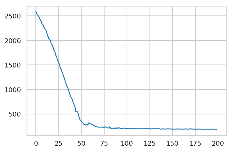
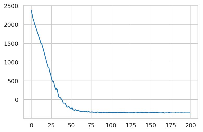
Minimalkan kerugian variasi.
# Allow external control of optimization to reduce test runtimes.
num_variational_steps = 200 # @param { isTemplate: true}
num_variational_steps = int(num_variational_steps)

# Build and optimize the variational loss function.
elbo_loss_curve = tfp.vi.fit_surrogate_posterior(
    target_log_prob_fn=co2_model.joint_distribution(
        observed_time_series=co2_by_month_training_data).log_prob,
    surrogate_posterior=variational_posteriors,
    optimizer=tf.optimizers.Adam(learning_rate=0.1),
    num_steps=num_variational_steps,
    jit_compile=True)

plt.plot(elbo_loss_curve)
plt.show()

# Draw samples from the variational posterior.
q_samples_co2_ = variational_posteriors.sample(50)
WARNING:tensorflow:From /usr/local/lib/python3.6/dist-packages/tensorflow_core/python/ops/linalg/linear_operator_diag.py:166: calling LinearOperator.__init__ (from tensorflow.python.ops.linalg.linear_operator) with graph_parents is deprecated and will be removed in a future version.
Instructions for updating:
Do not pass `graph_parents`.  They will  no longer be used.
print("Inferred parameters:")
for param in co2_model.parameters:
  print("{}: {} +- {}".format(param.name,
                              np.mean(q_samples_co2_[param.name], axis=0),
                              np.std(q_samples_co2_[param.name], axis=0)))
Inferred parameters:
observation_noise_scale: 0.17199112474918365 +- 0.009443143382668495
LocalLinearTrend/_level_scale: 0.17671072483062744 +- 0.01510554924607277
LocalLinearTrend/_slope_scale: 0.004302256740629673 +- 0.0018349259626120329
Seasonal/_drift_scale: 0.041069451719522476 +- 0.007772190496325493
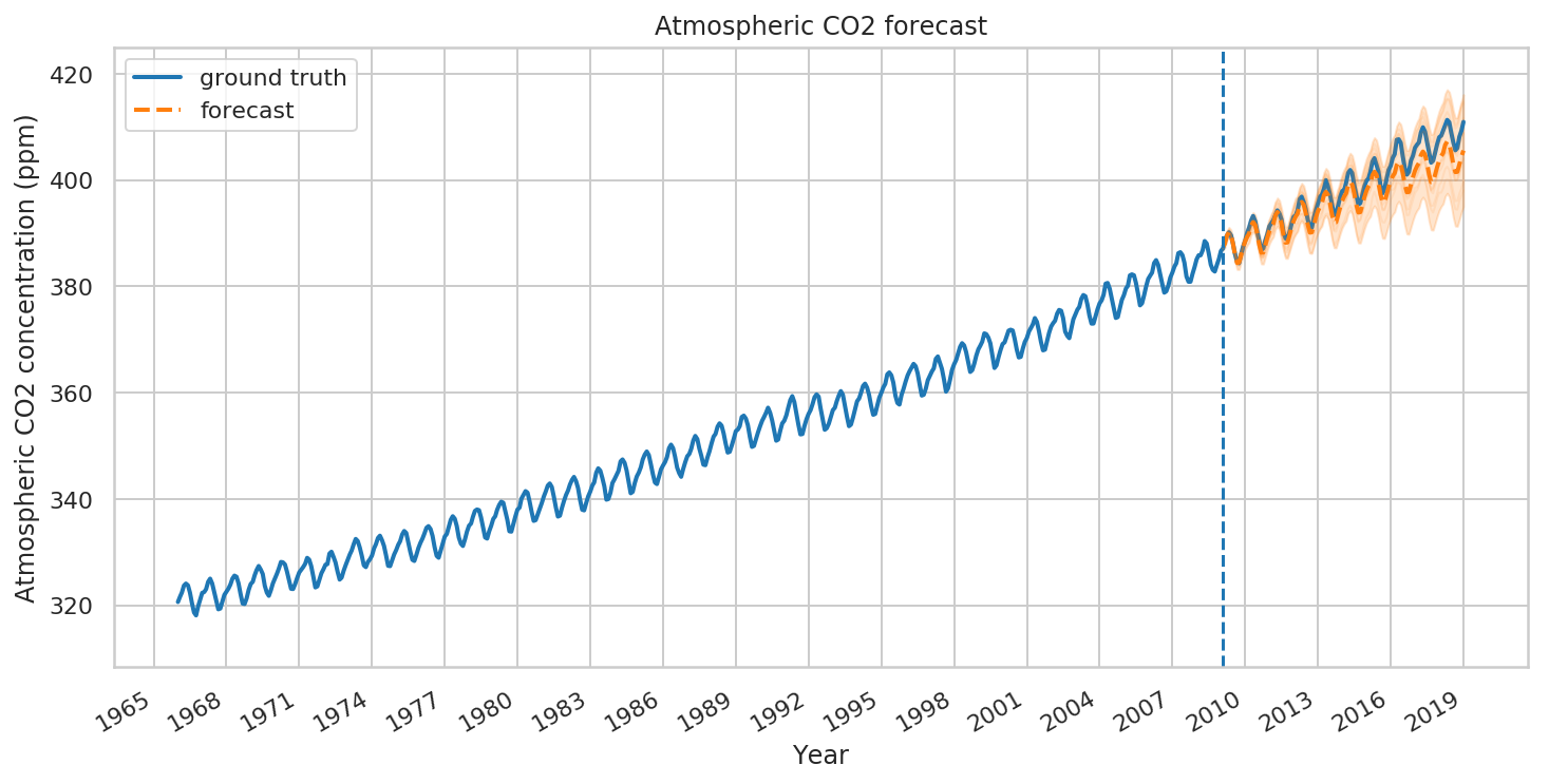
Ramalan dan kritik
Sekarang mari kita gunakan model yang pas untuk membuat ramalan. Kami hanya memanggil tfp.sts.forecast , yang mengembalikan instans Distribusi TensorFlow yang mewakili distribusi prediktif selama langkah waktu mendatang.
co2_forecast_dist = tfp.sts.forecast(
    co2_model,
    observed_time_series=co2_by_month_training_data,
    parameter_samples=q_samples_co2_,
    num_steps_forecast=num_forecast_steps)
Secara khusus, mean dan stddev dari distribusi ramalan memberi kita prediksi dengan ketidakpastian marjinal pada setiap langkah waktu, dan kita juga dapat menarik sampel kemungkinan masa depan.
num_samples=10

co2_forecast_mean, co2_forecast_scale, co2_forecast_samples = (
    co2_forecast_dist.mean().numpy()[..., 0],
    co2_forecast_dist.stddev().numpy()[..., 0],
    co2_forecast_dist.sample(num_samples).numpy()[..., 0])
fig, ax = plot_forecast(
    co2_dates, co2_by_month,
    co2_forecast_mean, co2_forecast_scale, co2_forecast_samples,
    x_locator=co2_loc,
    x_formatter=co2_fmt,
    title="Atmospheric CO2 forecast")
ax.axvline(co2_dates[-num_forecast_steps], linestyle="--")
ax.legend(loc="upper left")
ax.set_ylabel("Atmospheric CO2 concentration (ppm)")
ax.set_xlabel("Year")
fig.autofmt_xdate()
Kita dapat lebih memahami kecocokan model dengan menguraikannya menjadi kontribusi deret waktu individu:
# Build a dict mapping components to distributions over
# their contribution to the observed signal.
component_dists = sts.decompose_by_component(
    co2_model,
    observed_time_series=co2_by_month,
    parameter_samples=q_samples_co2_)
co2_component_means_, co2_component_stddevs_ = (
    {k.name: c.mean() for k, c in component_dists.items()},
    {k.name: c.stddev() for k, c in component_dists.items()})
_ = plot_components(co2_dates, co2_component_means_, co2_component_stddevs_,
                    x_locator=co2_loc, x_formatter=co2_fmt)
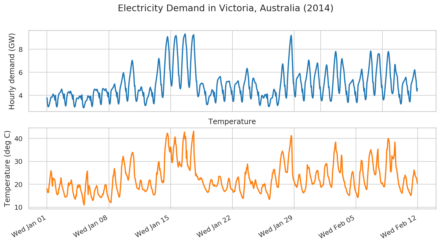
Prakiraan permintaan listrik
Sekarang mari kita perhatikan contoh yang lebih kompleks: meramalkan permintaan listrik di Victoria Australia.
Pertama, kita akan membangun kumpulan data:
# Victoria electricity demand dataset, as presented at
# https://otexts.com/fpp2/scatterplots.html
# and downloaded from https://github.com/robjhyndman/fpp2-package/blob/master/data/elecdaily.rda
# This series contains the first eight weeks (starting Jan 1). The original
# dataset was half-hourly data; here we've downsampled to hourly data by taking
# every other timestep.
demand_dates = np.arange('2014-01-01', '2014-02-26', dtype='datetime64[h]')
demand_loc = mdates.WeekdayLocator(byweekday=mdates.WE)
demand_fmt = mdates.DateFormatter('%a %b %d')

demand = np.array("3.794,3.418,3.152,3.026,3.022,3.055,3.180,3.276,3.467,3.620,3.730,3.858,3.851,3.839,3.861,3.912,4.082,4.118,4.011,3.965,3.932,3.693,3.585,4.001,3.623,3.249,3.047,3.004,3.104,3.361,3.749,3.910,4.075,4.165,4.202,4.225,4.265,4.301,4.381,4.484,4.552,4.440,4.233,4.145,4.116,3.831,3.712,4.121,3.764,3.394,3.159,3.081,3.216,3.468,3.838,4.012,4.183,4.269,4.280,4.310,4.315,4.233,4.188,4.263,4.370,4.308,4.182,4.075,4.057,3.791,3.667,4.036,3.636,3.283,3.073,3.003,3.023,3.113,3.335,3.484,3.697,3.723,3.786,3.763,3.748,3.714,3.737,3.828,3.937,3.929,3.877,3.829,3.950,3.756,3.638,4.045,3.682,3.283,3.036,2.933,2.956,2.959,3.157,3.236,3.370,3.493,3.516,3.555,3.570,3.656,3.792,3.950,3.953,3.926,3.849,3.813,3.891,3.683,3.562,3.936,3.602,3.271,3.085,3.041,3.201,3.570,4.123,4.307,4.481,4.533,4.545,4.524,4.470,4.457,4.418,4.453,4.539,4.473,4.301,4.260,4.276,3.958,3.796,4.180,3.843,3.465,3.246,3.203,3.360,3.808,4.328,4.509,4.598,4.562,4.566,4.532,4.477,4.442,4.424,4.486,4.579,4.466,4.338,4.270,4.296,4.034,3.877,4.246,3.883,3.520,3.306,3.252,3.387,3.784,4.335,4.465,4.529,4.536,4.589,4.660,4.691,4.747,4.819,4.950,4.994,4.798,4.540,4.352,4.370,4.047,3.870,4.245,3.848,3.509,3.302,3.258,3.419,3.809,4.363,4.605,4.793,4.908,5.040,5.204,5.358,5.538,5.708,5.888,5.966,5.817,5.571,5.321,5.141,4.686,4.367,4.618,4.158,3.771,3.555,3.497,3.646,4.053,4.687,5.052,5.342,5.586,5.808,6.038,6.296,6.548,6.787,6.982,7.035,6.855,6.561,6.181,5.899,5.304,4.795,4.862,4.264,3.820,3.588,3.481,3.514,3.632,3.857,4.116,4.375,4.462,4.460,4.422,4.398,4.407,4.480,4.621,4.732,4.735,4.572,4.385,4.323,4.069,3.940,4.247,3.821,3.416,3.220,3.124,3.132,3.181,3.337,3.469,3.668,3.788,3.834,3.894,3.964,4.109,4.275,4.472,4.623,4.703,4.594,4.447,4.459,4.137,3.913,4.231,3.833,3.475,3.302,3.279,3.519,3.975,4.600,4.864,5.104,5.308,5.542,5.759,6.005,6.285,6.617,6.993,7.207,7.095,6.839,6.387,6.048,5.433,4.904,4.959,4.425,4.053,3.843,3.823,4.017,4.521,5.229,5.802,6.449,6.975,7.506,7.973,8.359,8.596,8.794,9.030,9.090,8.885,8.525,8.147,7.797,6.938,6.215,6.123,5.495,5.140,4.896,4.812,5.024,5.536,6.293,7.000,7.633,8.030,8.459,8.768,9.000,9.113,9.155,9.173,9.039,8.606,8.095,7.617,7.208,6.448,5.740,5.718,5.106,4.763,4.610,4.566,4.737,5.204,5.988,6.698,7.438,8.040,8.484,8.837,9.052,9.114,9.214,9.307,9.313,9.006,8.556,8.275,7.911,7.077,6.348,6.175,5.455,5.041,4.759,4.683,4.908,5.411,6.199,6.923,7.593,8.090,8.497,8.843,9.058,9.159,9.231,9.253,8.852,7.994,7.388,6.735,6.264,5.690,5.227,5.220,4.593,4.213,3.984,3.891,3.919,4.031,4.287,4.558,4.872,4.963,5.004,5.017,5.057,5.064,5.000,5.023,5.007,4.923,4.740,4.586,4.517,4.236,4.055,4.337,3.848,3.473,3.273,3.198,3.204,3.252,3.404,3.560,3.767,3.896,3.934,3.972,3.985,4.032,4.122,4.239,4.389,4.499,4.406,4.356,4.396,4.106,3.914,4.265,3.862,3.546,3.360,3.359,3.649,4.180,4.813,5.086,5.301,5.384,5.434,5.470,5.529,5.582,5.618,5.636,5.561,5.291,5.000,4.840,4.767,4.364,4.160,4.452,4.011,3.673,3.503,3.483,3.695,4.213,4.810,5.028,5.149,5.182,5.208,5.179,5.190,5.220,5.202,5.216,5.232,5.019,4.828,4.686,4.657,4.304,4.106,4.389,3.955,3.643,3.489,3.479,3.695,4.187,4.732,4.898,4.997,5.001,5.022,5.052,5.094,5.143,5.178,5.250,5.255,5.075,4.867,4.691,4.665,4.352,4.121,4.391,3.966,3.615,3.437,3.430,3.666,4.149,4.674,4.851,5.011,5.105,5.242,5.378,5.576,5.790,6.030,6.254,6.340,6.253,6.039,5.736,5.490,4.936,4.580,4.742,4.230,3.895,3.712,3.700,3.906,4.364,4.962,5.261,5.463,5.495,5.477,5.394,5.250,5.159,5.081,5.083,5.038,4.857,4.643,4.526,4.428,4.141,3.975,4.290,3.809,3.423,3.217,3.132,3.192,3.343,3.606,3.803,3.963,3.998,3.962,3.894,3.814,3.776,3.808,3.914,4.033,4.079,4.027,3.974,4.057,3.859,3.759,4.132,3.716,3.325,3.111,3.030,3.046,3.096,3.254,3.390,3.606,3.718,3.755,3.768,3.768,3.834,3.957,4.199,4.393,4.532,4.516,4.380,4.390,4.142,3.954,4.233,3.795,3.425,3.209,3.124,3.177,3.288,3.498,3.715,4.092,4.383,4.644,4.909,5.184,5.518,5.889,6.288,6.643,6.729,6.567,6.179,5.903,5.278,4.788,4.885,4.363,4.011,3.823,3.762,3.998,4.598,5.349,5.898,6.487,6.941,7.381,7.796,8.185,8.522,8.825,9.103,9.198,8.889,8.174,7.214,6.481,5.611,5.026,5.052,4.484,4.148,3.955,3.873,4.060,4.626,5.272,5.441,5.535,5.534,5.610,5.671,5.724,5.793,5.838,5.908,5.868,5.574,5.276,5.065,4.976,4.554,4.282,4.547,4.053,3.720,3.536,3.524,3.792,4.420,5.075,5.208,5.344,5.482,5.701,5.936,6.210,6.462,6.683,6.979,7.059,6.893,6.535,6.121,5.797,5.152,4.705,4.805,4.272,3.975,3.805,3.775,3.996,4.535,5.275,5.509,5.730,5.870,6.034,6.175,6.340,6.500,6.603,6.804,6.787,6.460,6.043,5.627,5.367,4.866,4.575,4.728,4.157,3.795,3.607,3.537,3.596,3.803,4.125,4.398,4.660,4.853,5.115,5.412,5.669,5.930,6.216,6.466,6.641,6.605,6.316,5.821,5.520,5.016,4.657,4.746,4.197,3.823,3.613,3.505,3.488,3.532,3.716,4.011,4.421,4.836,5.296,5.766,6.233,6.646,7.011,7.380,7.660,7.804,7.691,7.364,7.019,6.260,5.545,5.437,4.806,4.457,4.235,4.172,4.396,5.002,5.817,6.266,6.732,7.049,7.184,7.085,6.798,6.632,6.408,6.218,5.968,5.544,5.217,4.964,4.758,4.328,4.074,4.367,3.883,3.536,3.404,3.396,3.624,4.271,4.916,4.953,5.016,5.048,5.106,5.124,5.200,5.244,5.242,5.341,5.368,5.166,4.910,4.762,4.700,4.276,4.035,4.318,3.858,3.550,3.399,3.382,3.590,4.261,4.937,4.994,5.094,5.168,5.303,5.410,5.571,5.740,5.900,6.177,6.274,6.039,5.700,5.389,5.192,4.672,4.359,4.614,4.118,3.805,3.627,3.646,3.882,4.470,5.106,5.274,5.507,5.711,5.950,6.200,6.527,6.884,7.196,7.615,7.845,7.759,7.437,7.059,6.584,5.742,5.125,5.139,4.564,4.218,4.025,4.000,4.245,4.783,5.504,5.920,6.271,6.549,6.894,7.231,7.535,7.597,7.562,7.609,7.534,7.118,6.448,5.963,5.565,5.005,4.666,4.850,4.302,3.905,3.678,3.610,3.672,3.869,4.204,4.541,4.944,5.265,5.651,6.090,6.547,6.935,7.318,7.625,7.793,7.760,7.510,7.145,6.805,6.103,5.520,5.462,4.824,4.444,4.237,4.157,4.164,4.275,4.545,5.033,5.594,6.176,6.681,6.628,6.238,6.039,5.897,5.832,5.701,5.483,4.949,4.589,4.407,4.027,3.820,4.075,3.650,3.388,3.271,3.268,3.498,4.086,4.800,4.933,5.102,5.126,5.194,5.260,5.319,5.364,5.419,5.559,5.568,5.332,5.027,4.864,4.738,4.303,4.093,4.379,3.952,3.632,3.461,3.446,3.732,4.294,4.911,5.021,5.138,5.223,5.348,5.479,5.661,5.832,5.966,6.178,6.212,5.949,5.640,5.449,5.213,4.678,4.376,4.601,4.147,3.815,3.610,3.605,3.879,4.468,5.090,5.226,5.406,5.561,5.740,5.899,6.095,6.272,6.402,6.610,6.585,6.265,5.925,5.747,5.497,4.932,4.580,4.763,4.298,4.026,3.871,3.827,4.065,4.643,5.317,5.494,5.685,5.814,5.912,5.999,6.097,6.176,6.136,6.131,6.049,5.796,5.532,5.475,5.254,4.742,4.453,4.660,4.176,3.895,3.726,3.717,3.910,4.479,5.135,5.306,5.520,5.672,5.737,5.785,5.829,5.893,5.892,5.921,5.817,5.557,5.304,5.234,5.074,4.656,4.396,4.599,4.064,3.749,3.560,3.475,3.552,3.783,4.045,4.258,4.539,4.762,4.938,5.049,5.037,5.066,5.151,5.197,5.201,5.132,4.908,4.725,4.568,4.222,3.939,4.215,3.741,3.380,3.174,3.076,3.071,3.172,3.328,3.427,3.603,3.738,3.765,3.777,3.705,3.690,3.742,3.859,4.032,4.113,4.032,4.066,4.011,3.712,3.530,3.905,3.556,3.283,3.136,3.146,3.400,4.009,4.717,4.827,4.909,4.973,5.036,5.079,5.160,5.228,5.241,5.343,5.350,5.184,4.941,4.797,4.615,4.160,3.904,4.213,3.810,3.528,3.369,3.381,3.609,4.178,4.861,4.918,5.006,5.102,5.239,5.385,5.528,5.724,5.845,6.048,6.097,5.838,5.507,5.267,5.003,4.462,4.184,4.431,3.969,3.660,3.480,3.470,3.693,4.313,4.955,5.083,5.251,5.268,5.293,5.285,5.308,5.349,5.322,5.328,5.151,4.975,4.741,4.678,4.458,4.056,3.868,4.226,3.799,3.428,3.253,3.228,3.452,4.040,4.726,4.709,4.721,4.741,4.846,4.864,4.868,4.836,4.799,4.890,4.946,4.800,4.646,4.693,4.546,4.117,3.897,4.259,3.893,3.505,3.341,3.334,3.623,4.240,4.925,4.986,5.028,4.987,4.984,4.975,4.912,4.833,4.686,4.710,4.718,4.577,4.454,4.532,4.407,4.064,3.883,4.221,3.792,3.445,3.261,3.221,3.295,3.521,3.804,4.038,4.200,4.226,4.198,4.182,4.078,4.018,4.002,4.066,4.158,4.154,4.084,4.104,4.001,3.773,3.700,4.078,3.702,3.349,3.143,3.052,3.070,3.181,3.327,3.440,3.616,3.678,3.694,3.710,3.706,3.764,3.852,4.009,4.202,4.323,4.249,4.275,4.162,3.848,3.706,4.060,3.703,3.401,3.251,3.239,3.455,4.041,4.743,4.815,4.916,4.931,4.966,5.063,5.218,5.381,5.458,5.550,5.566,5.376,5.104,5.022,4.793,4.335,4.108,4.410,4.008,3.666,3.497,3.464,3.698,4.333,4.998,5.094,5.272,5.459,5.648,5.853,6.062,6.258,6.236,6.226,5.957,5.455,5.066,4.968,4.742,4.304,4.105,4.410".split(",")).astype(np.float32)
temperature = np.array("18.050,17.200,16.450,16.650,16.400,17.950,19.700,20.600,22.350,23.700,24.800,25.900,25.300,23.650,20.700,19.150,22.650,22.650,22.400,22.150,22.050,22.150,21.000,19.500,18.450,17.250,16.300,15.700,15.500,15.450,15.650,16.500,18.100,17.800,19.100,19.850,20.300,21.050,22.800,21.650,20.150,19.300,18.750,17.900,17.350,16.850,16.350,15.700,14.950,14.500,14.350,14.450,14.600,14.600,14.700,15.450,16.700,18.300,20.100,20.650,19.450,20.200,20.250,20.050,20.250,20.950,21.900,21.000,19.900,19.250,17.300,16.300,15.800,15.000,14.400,14.050,13.650,13.500,14.150,15.300,14.800,17.050,18.350,19.450,18.550,18.650,18.850,19.800,19.650,18.900,19.500,17.700,17.350,16.950,16.400,15.950,14.900,14.250,13.050,12.000,11.500,10.950,12.300,16.100,17.100,19.600,21.100,22.600,24.350,25.250,25.750,20.350,15.550,18.300,19.400,19.250,18.550,17.700,16.750,15.800,14.900,14.050,14.100,13.500,13.000,12.950,13.300,13.900,15.400,16.750,17.300,17.750,18.400,18.500,18.800,19.450,18.750,18.400,16.950,15.800,15.350,15.250,15.150,14.900,14.500,14.600,14.400,14.150,14.300,14.500,14.950,15.550,15.800,15.550,16.450,17.500,17.700,18.750,19.600,19.900,19.350,19.550,17.900,16.400,15.550,14.900,14.400,13.950,13.300,12.950,12.650,12.450,12.350,12.150,11.950,14.150,15.850,17.750,19.450,22.150,23.850,23.450,24.950,26.850,26.100,25.150,23.250,21.300,19.850,18.900,18.250,17.450,17.100,16.400,15.550,15.050,14.400,14.550,15.150,17.050,18.850,20.850,24.250,27.700,28.400,30.750,30.700,32.200,31.750,30.650,29.750,28.850,27.850,25.950,24.700,24.850,24.050,23.850,23.500,22.950,22.200,21.750,22.350,24.050,25.150,27.100,28.050,29.750,31.250,31.900,32.950,33.150,33.950,33.850,33.250,32.500,31.500,28.300,23.900,22.900,22.300,21.250,20.500,19.850,18.850,18.300,18.100,18.200,18.150,18.000,17.700,18.250,19.700,20.750,21.800,21.500,21.600,20.800,19.400,18.400,17.900,17.600,17.550,17.550,17.650,17.400,17.150,16.800,17.000,16.900,17.200,17.350,17.650,17.800,18.400,19.300,20.200,21.050,21.700,21.800,21.800,21.500,20.000,19.300,18.200,18.100,17.700,16.950,16.250,15.600,15.500,15.300,15.450,15.500,15.750,17.350,19.150,21.650,24.700,25.200,24.300,26.900,28.100,29.450,29.850,29.450,26.350,27.050,25.700,25.150,23.850,22.450,21.450,20.850,20.700,21.300,21.550,20.800,22.300,26.300,32.600,35.150,36.800,38.150,39.950,40.850,41.250,42.300,41.950,41.350,40.600,36.350,36.150,34.600,34.050,35.400,36.300,35.550,33.700,30.650,29.450,29.500,31.000,33.300,35.700,36.650,37.650,39.400,40.600,40.250,37.550,37.300,35.400,32.750,31.200,29.600,28.350,27.500,28.750,28.900,29.900,28.700,28.650,28.150,28.250,27.650,27.800,29.450,32.500,35.750,38.850,39.900,41.100,41.800,42.750,39.900,39.750,40.800,37.950,31.250,34.600,30.250,28.500,27.900,27.950,27.300,26.900,26.800,26.050,26.100,27.700,31.850,34.850,36.350,38.000,39.200,41.050,41.600,42.350,43.100,33.500,30.700,29.100,26.400,23.900,24.700,24.350,23.450,23.450,23.550,23.050,22.200,22.100,22.000,21.900,22.050,22.550,22.850,22.450,22.250,22.650,22.350,21.900,21.000,20.950,20.200,19.700,19.400,19.200,18.650,18.150,18.150,17.650,17.350,17.150,16.800,16.750,16.400,16.500,16.700,17.300,17.750,19.200,20.400,20.900,21.450,22.000,22.100,21.600,21.700,20.500,19.850,19.750,19.500,19.200,19.800,19.500,19.200,19.200,19.150,19.050,19.100,19.250,19.550,20.200,20.550,21.450,23.150,23.500,23.400,23.500,23.300,22.850,22.250,20.950,19.750,19.450,18.900,18.450,17.950,17.550,17.300,16.950,16.900,16.850,17.100,17.250,17.400,17.850,18.100,18.600,19.700,21.000,21.400,22.650,22.550,22.000,21.050,19.550,18.550,18.300,17.750,17.800,17.650,17.800,17.450,16.950,16.500,16.900,17.050,16.750,17.300,18.800,19.350,20.750,21.400,21.900,21.950,22.800,22.750,23.200,22.650,20.800,19.250,17.800,16.950,16.550,16.050,15.750,15.150,14.700,14.150,13.900,13.900,14.000,15.800,17.650,19.700,22.500,25.300,24.300,24.650,26.450,27.250,26.550,28.800,27.850,25.200,24.750,23.750,22.550,22.350,21.700,21.300,20.300,20.050,20.500,21.250,20.850,21.000,19.400,18.900,18.150,18.650,20.200,20.000,21.650,21.950,21.150,20.400,19.500,19.150,18.400,18.050,17.750,17.600,17.150,16.750,16.350,16.250,15.900,15.850,15.900,16.200,18.500,18.750,18.800,19.850,19.750,19.600,19.300,20.000,20.250,19.700,18.600,17.400,17.100,16.650,16.250,16.250,15.800,15.350,14.800,14.250,13.500,13.400,14.350,15.800,17.700,19.000,21.050,22.200,22.450,24.950,24.750,25.050,26.400,26.200,26.500,25.850,24.400,23.600,22.650,21.500,20.150,19.900,18.850,18.700,18.750,18.650,20.050,23.450,24.900,26.450,28.550,30.600,31.550,32.800,33.500,33.700,34.450,34.200,33.650,32.900,31.750,30.500,29.250,28.100,26.450,25.400,25.400,25.150,25.400,25.100,25.950,28.100,30.400,32.000,33.750,34.700,35.800,37.000,39.050,39.750,41.200,41.050,36.050,28.250,24.450,23.150,22.050,21.600,21.450,20.800,20.250,19.700,19.400,19.650,19.100,18.650,18.900,19.400,20.700,21.750,22.350,24.100,23.350,24.400,22.950,22.400,20.950,19.600,18.900,18.000,17.400,16.800,16.550,16.300,16.250,16.750,16.700,17.100,17.500,18.150,18.850,20.650,22.600,25.600,28.500,26.750,27.200,27.300,27.500,27.000,25.450,24.500,23.850,23.200,22.550,21.850,21.050,20.200,19.950,20.400,20.300,20.100,20.450,20.900,21.450,21.800,23.250,24.100,25.200,25.550,25.900,25.450,26.050,25.350,23.900,22.250,22.000,21.700,21.450,20.550,19.000,18.850,18.700,19.050,19.350,19.350,19.450,19.600,20.550,22.400,24.550,26.900,27.950,28.500,28.200,29.050,28.700,28.800,27.150,24.900,23.500,23.350,23.000,22.300,21.400,20.700,19.850,19.400,19.250,18.700,18.650,20.200,23.400,26.400,27.450,29.150,32.050,34.500,34.950,36.550,37.850,38.400,35.150,34.050,34.100,33.100,30.300,29.300,27.550,26.600,25.900,25.500,25.150,25.000,25.150,27.000,31.150,32.750,31.500,26.900,23.900,23.150,22.850,21.500,21.150,21.300,19.700,18.800,18.450,18.300,17.800,16.850,16.400,16.150,15.700,15.500,15.400,15.300,15.050,15.650,18.100,19.200,21.050,22.350,23.450,24.850,24.950,25.550,25.300,24.250,22.750,20.850,19.350,18.250,17.450,17.000,16.500,16.100,15.950,15.300,14.550,14.250,14.400,15.550,18.300,20.000,22.750,25.450,25.800,26.350,29.150,30.450,30.350,29.600,27.550,25.550,23.650,22.950,21.850,20.700,20.150,19.300,19.000,18.400,17.800,17.750,18.000,20.800,23.400,25.750,27.750,29.600,32.150,32.900,33.650,34.300,34.800,35.050,33.750,33.250,32.400,31.250,29.650,28.550,26.550,25.950,25.000,24.400,24.150,24.150,24.350,26.900,28.750,30.350,32.750,34.250,35.300,28.400,27.250,26.600,25.750,25.350,23.150,21.550,20.850,20.550,20.350,20.550,20.600,19.900,19.550,19.200,18.900,18.850,19.250,21.000,23.050,25.350,27.700,31.050,35.250,35.100,36.850,39.250,40.000,39.450,38.950,37.750,33.850,30.400,25.700,25.400,25.600,28.150,32.400,31.850,31.350,31.200,31.100,31.950,32.450,35.200,38.400,35.850,30.700,27.850,26.900,26.650,25.250,24.450,22.500,22.050,20.000,19.750,19.100,18.500,18.400,17.400,16.900,16.800,16.450,16.050,16.300,17.450,19.300,20.000,21.050,22.800,22.550,23.300,24.050,23.100,23.100,22.500,20.800,19.550,18.800,18.200,17.650,17.750,17.150,16.550,16.200,16.000,15.600,15.150,15.150,16.250,17.800,19.150,21.000,22.800,23.850,24.250,26.200,25.650,25.050,23.850,23.600,23.100,22.950,22.550,21.550,20.450,19.600,18.700,18.300,18.000,17.550,17.300,17.200,17.950,19.450,21.100,23.050,24.650,25.050,25.850,25.300,26.650,25.500,25.900,26.250,25.300,25.150,23.600,22.050,21.700,21.150,20.550,20.500,20.200,20.500,20.600,20.900,21.700,22.000,22.250,23.400,23.900,25.250,26.200,26.000,25.300,25.200,25.300,25.500,25.350,25.050,24.850,24.050,23.150,22.300,21.900,21.150,20.300,19.650,19.700,19.750,20.250,21.500,23.600,24.600,25.900,25.450,24.850,25.900,26.150,26.250,26.350,26.250,25.850,25.300,24.600,23.750,22.250,21.750,21.450,21.500,21.300,21.250,21.200,21.600,22.000,23.650,25.200,26.400,25.500,25.150,26.950,28.350,25.650,25.000,25.500,24.150,22.900,21.600,21.750,21.500,21.550,20.450,19.500,18.750,18.650,18.200,17.300,17.900,18.050,17.400,16.850,17.950,20.550,21.950,22.600,22.300,22.400,22.300,21.100,20.250,19.200,18.900,18.600,18.350,17.700,17.200,16.850,16.900,16.800,16.800,16.600,16.350,17.200,18.350,19.550,20.300,21.600,21.800,23.300,23.200,24.550,24.950,24.900,23.700,22.000,19.650,18.250,17.700,17.250,16.900,16.550,16.050,16.450,15.400,14.900,14.700,16.100,18.450,19.800,23.000,25.250,27.600,27.900,28.550,29.450,29.700,29.350,27.000,23.550,21.900,20.750,20.150,19.600,19.150,18.800,18.550,18.200,17.750,17.650,17.800,18.750,19.600,20.450,21.950,23.700,23.150,24.150,24.550,21.400,19.150,19.050,16.500,15.900,14.850,15.300,14.100,13.800,13.600,13.450,13.400,13.050,12.750,12.800,12.750,13.600,14.950,16.100,17.500,18.500,19.300,19.400,19.750,19.400,19.450,19.450,18.900,17.650,16.800,15.900,15.050,14.550,14.250,13.800,13.850,13.700,13.650,13.350,13.400,14.050,15.000,16.650,17.850,18.450,18.200,18.900,19.850,20.000,19.700,18.800,17.500,16.600,16.250,16.000,16.300,16.400,15.800,15.850,14.600,14.650,15.200,14.900,14.600,15.150,16.000,16.350,17.000,18.300,19.050,19.300,19.400,18.650,18.750,19.100,18.300,17.950,17.550,16.900,16.450,15.850,15.800,15.650,15.200,14.700,14.950,15.250,15.200,15.800,16.800,17.900,19.700,21.050,21.600,22.550,22.750,22.900,22.500,21.950,20.450,19.600,19.200,18.000,16.950,16.450,16.150,15.600,15.150,15.250,15.200,14.750,15.050,15.600,17.750,18.450,20.050,21.350,22.500,23.550,24.100,22.600,23.150,24.100,22.650,21.250,19.900,19.100,18.250,17.750,17.500,16.600,16.100,15.850,15.750,15.700,16.350,19.600,25.750,27.800,30.050,32.350,31.900,32.450,29.600,28.850,23.450,21.100,20.100,20.100,19.900,19.300,19.050,18.850".split(",")).astype(np.float32)

num_forecast_steps = 24 * 7 * 2 # Two weeks.
demand_training_data = demand[:-num_forecast_steps]
colors = sns.color_palette()
c1, c2 = colors[0], colors[1]

fig = plt.figure(figsize=(12, 6))
ax = fig.add_subplot(2, 1, 1)
ax.plot(demand_dates[:-num_forecast_steps],
        demand[:-num_forecast_steps], lw=2, label="training data")
ax.set_ylabel("Hourly demand (GW)")

ax = fig.add_subplot(2, 1, 2)

ax.plot(demand_dates[:-num_forecast_steps],
        temperature[:-num_forecast_steps], lw=2, label="training data", c=c2)
ax.set_ylabel("Temperature (deg C)")
ax.set_title("Temperature")
ax.xaxis.set_major_locator(demand_loc)
ax.xaxis.set_major_formatter(demand_fmt)
fig.suptitle("Electricity Demand in Victoria, Australia (2014)",
             fontsize=15)
fig.autofmt_xdate()
Model dan pas
Model kami menggabungkan musiman jam-hari dan hari-minggu, dengan pemodelan regresi linier efek suhu, dan proses autoregresif untuk menangani residual varians terbatas.
def build_model(observed_time_series):
  hour_of_day_effect = sts.Seasonal(
      num_seasons=24,
      observed_time_series=observed_time_series,
      name='hour_of_day_effect')
  day_of_week_effect = sts.Seasonal(
      num_seasons=7, num_steps_per_season=24,
      observed_time_series=observed_time_series,
      name='day_of_week_effect')
  temperature_effect = sts.LinearRegression(
      design_matrix=tf.reshape(temperature - np.mean(temperature),
                               (-1, 1)), name='temperature_effect')
  autoregressive = sts.Autoregressive(
      order=1,
      observed_time_series=observed_time_series,
      name='autoregressive')
  model = sts.Sum([hour_of_day_effect,
                   day_of_week_effect,
                   temperature_effect,
                   autoregressive],
                   observed_time_series=observed_time_series)
  return model
Seperti di atas, kita akan menyesuaikan model dengan inferensi variasi dan menarik sampel dari posterior.
demand_model = build_model(demand_training_data)

# Build the variational surrogate posteriors `qs`.
variational_posteriors = tfp.sts.build_factored_surrogate_posterior(
    model=demand_model)
Minimalkan kerugian variasi.
# Allow external control of optimization to reduce test runtimes.
num_variational_steps = 200 # @param { isTemplate: true}
num_variational_steps = int(num_variational_steps)

# Build and optimize the variational loss function.
elbo_loss_curve = tfp.vi.fit_surrogate_posterior(
    target_log_prob_fn=demand_model.joint_distribution(
        observed_time_series=demand_training_data).log_prob,
    surrogate_posterior=variational_posteriors,
    optimizer=tf.optimizers.Adam(learning_rate=0.1),
    num_steps=num_variational_steps,
    jit_compile=True)
plt.plot(elbo_loss_curve)
plt.show()

# Draw samples from the variational posterior.
q_samples_demand_ = variational_posteriors.sample(50)
print("Inferred parameters:")
for param in demand_model.parameters:
  print("{}: {} +- {}".format(param.name,
                              np.mean(q_samples_demand_[param.name], axis=0),
                              np.std(q_samples_demand_[param.name], axis=0)))
Inferred parameters:
observation_noise_scale: 0.010157477110624313 +- 0.0026443174574524164
hour_of_day_effect/_drift_scale: 0.0019522204529494047 +- 0.0011986979516223073
day_of_week_effect/_drift_scale: 0.013334915973246098 +- 0.01825258508324623
temperature_effect/_weights: [0.06648794] +- [0.00411669]
autoregressive/_coefficients: [0.9871232] +- [0.00413899]
autoregressive/_level_scale: 0.14199139177799225 +- 0.002658574376255274
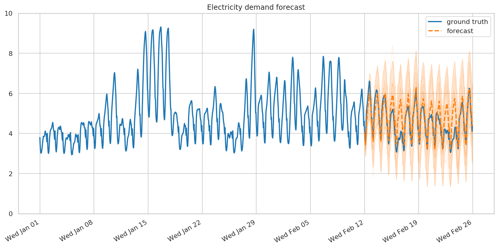
Ramalan dan kritik
Sekali lagi, kami membuat perkiraan hanya dengan memanggil tfp.sts.forecast dengan model, deret waktu, dan parameter sampel kami.
demand_forecast_dist = tfp.sts.forecast(
    model=demand_model,
    observed_time_series=demand_training_data,
    parameter_samples=q_samples_demand_,
    num_steps_forecast=num_forecast_steps)
num_samples=10

(
    demand_forecast_mean,
    demand_forecast_scale,
    demand_forecast_samples
) = (
    demand_forecast_dist.mean().numpy()[..., 0],
    demand_forecast_dist.stddev().numpy()[..., 0],
    demand_forecast_dist.sample(num_samples).numpy()[..., 0]
    )
fig, ax = plot_forecast(demand_dates, demand,
                        demand_forecast_mean,
                        demand_forecast_scale,
                        demand_forecast_samples,
                        title="Electricity demand forecast",
                        x_locator=demand_loc, x_formatter=demand_fmt)
ax.set_ylim([0, 10])
fig.tight_layout()
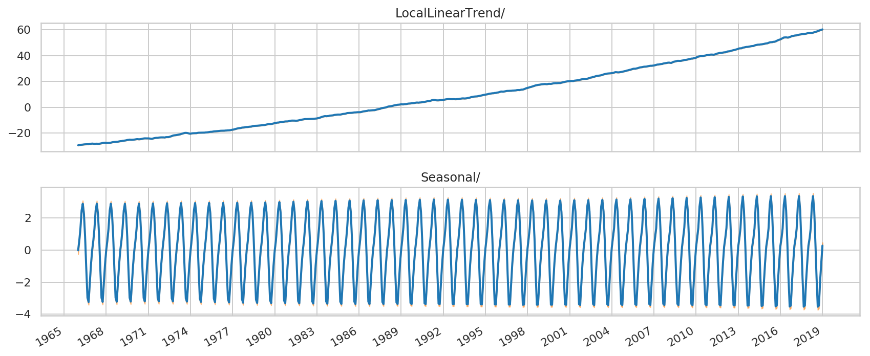
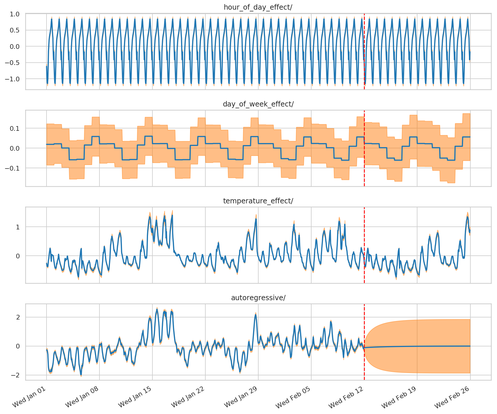
Mari kita visualisasikan dekomposisi rangkaian pengamatan dan perkiraan ke dalam komponen individu:
# Get the distributions over component outputs from the posterior marginals on
# training data, and from the forecast model.
component_dists = sts.decompose_by_component(
    demand_model,
    observed_time_series=demand_training_data,
    parameter_samples=q_samples_demand_)

forecast_component_dists = sts.decompose_forecast_by_component(
    demand_model,
    forecast_dist=demand_forecast_dist,
    parameter_samples=q_samples_demand_)
demand_component_means_, demand_component_stddevs_ = (
    {k.name: c.mean() for k, c in component_dists.items()},
    {k.name: c.stddev() for k, c in component_dists.items()})

(
    demand_forecast_component_means_,
    demand_forecast_component_stddevs_
) = (
    {k.name: c.mean() for k, c in forecast_component_dists.items()},
    {k.name: c.stddev() for k, c in forecast_component_dists.items()}
    )
# Concatenate the training data with forecasts for plotting.
component_with_forecast_means_ = collections.OrderedDict()
component_with_forecast_stddevs_ = collections.OrderedDict()
for k in demand_component_means_.keys():
  component_with_forecast_means_[k] = np.concatenate([
      demand_component_means_[k],
      demand_forecast_component_means_[k]], axis=-1)
  component_with_forecast_stddevs_[k] = np.concatenate([
      demand_component_stddevs_[k],
      demand_forecast_component_stddevs_[k]], axis=-1)


fig, axes = plot_components(
  demand_dates,
  component_with_forecast_means_,
  component_with_forecast_stddevs_,
  x_locator=demand_loc, x_formatter=demand_fmt)
for ax in axes.values():
  ax.axvline(demand_dates[-num_forecast_steps], linestyle="--", color='red')
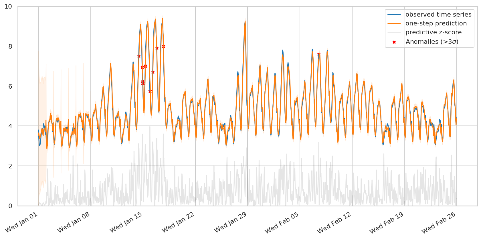
Jika kita ingin mendeteksi anomali dalam deret yang diamati, kita mungkin juga tertarik pada distribusi prediktif satu langkah: ramalan untuk setiap langkah waktu, yang diberikan hanya langkah waktu hingga titik itu. tfp.sts.one_step_predictive menghitung semua distribusi prediktif satu langkah dalam satu lintasan:
demand_one_step_dist = sts.one_step_predictive(
    demand_model,
    observed_time_series=demand,
    parameter_samples=q_samples_demand_)

demand_one_step_mean, demand_one_step_scale = (
    demand_one_step_dist.mean().numpy(), demand_one_step_dist.stddev().numpy())
Skema deteksi anomali sederhana adalah menandai semua langkah waktu di mana pengamatan lebih dari tiga stddev dari nilai yang diprediksi -- ini adalah langkah waktu yang paling 'mengejutkan' menurut model.
fig, ax = plot_one_step_predictive(
    demand_dates, demand,
    demand_one_step_mean, demand_one_step_scale,
    x_locator=demand_loc, x_formatter=demand_fmt)
ax.set_ylim(0, 10)

# Use the one-step-ahead forecasts to detect anomalous timesteps.
zscores = np.abs((demand - demand_one_step_mean) /
                 demand_one_step_scale)
anomalies = zscores > 3.0
ax.scatter(demand_dates[anomalies],
           demand[anomalies],
           c="red", marker="x", s=20, linewidth=2, label=r"Anomalies (>3$\sigma$)")
ax.plot(demand_dates, zscores, color="black", alpha=0.1, label='predictive z-score')
ax.legend()
plt.show()