
| | |  GitHub पर स्रोत देखें GitHub पर स्रोत देखें | |
TensorFlow संभावना (टीएफपी) संभाव्य तर्क और सांख्यिकीय विश्लेषण है कि अब भी पर काम करता है के लिए एक पुस्तकालय है JAX ! उन लोगों के लिए जो परिचित नहीं हैं, JAX कंपोज़ेबल फंक्शन ट्रांसफ़ॉर्मेशन के आधार पर त्वरित संख्यात्मक कंप्यूटिंग के लिए एक पुस्तकालय है।
जेएक्स पर टीएफपी नियमित टीएफपी की सबसे उपयोगी कार्यक्षमता का समर्थन करता है जबकि अमूर्त और एपीआई को संरक्षित करते हुए कई टीएफपी उपयोगकर्ता अब सहज हैं।
सेट अप
TFP JAX पर TensorFlow पर निर्भर नहीं करता; आइए इस Colab से TensorFlow को पूरी तरह से अनइंस्टॉल कर दें।
pip uninstall tensorflow -y -q
हम TFP के नवीनतम रात्रिकालीन निर्माण के साथ JAX पर TFP स्थापित कर सकते हैं।
pip install -Uq tfp-nightly[jax] > /dev/null
आइए कुछ उपयोगी पायथन पुस्तकालयों को आयात करें।
import matplotlib.pyplot as plt
import numpy as np
import seaborn as sns
from sklearn import datasets
sns.set(style='white')
/usr/local/lib/python3.6/dist-packages/statsmodels/tools/_testing.py:19: FutureWarning: pandas.util.testing is deprecated. Use the functions in the public API at pandas.testing instead.
  import pandas.util.testing as tm
आइए कुछ बुनियादी JAX कार्यक्षमता भी आयात करें।
import jax.numpy as jnp
from jax import grad
from jax import jit
from jax import random
from jax import value_and_grad
from jax import vmap
JAX . पर TFP आयात करना
JAX पर TFP का उपयोग करने के लिए बस आयात jax "सब्सट्रेट" और इसका इस्तेमाल के रूप में आप आमतौर पर होता tfp :
from tensorflow_probability.substrates import jax as tfp
tfd = tfp.distributions
tfb = tfp.bijectors
tfpk = tfp.math.psd_kernels
डेमो: बायेसियन लॉजिस्टिक रिग्रेशन
यह प्रदर्शित करने के लिए कि हम JAX बैकएंड के साथ क्या कर सकते हैं, हम क्लासिक आइरिस डेटासेट पर लागू बायेसियन लॉजिस्टिक रिग्रेशन को लागू करेंगे।
सबसे पहले, आइए आइरिस डेटासेट आयात करें और कुछ मेटाडेटा निकालें।
iris = datasets.load_iris()
features, labels = iris['data'], iris['target']

num_features = features.shape[-1]
num_classes = len(iris.target_names)
हम का उपयोग कर मॉडल को परिभाषित कर सकते tfd.JointDistributionCoroutine । हम दोनों वजन और पूर्वाग्रह अवधि पर मानक सामान्य महंतों डाल देता हूँ तो एक लिखने target_log_prob समारोह है कि पिन डेटा करने के लिए नमूने लेबल।
Root = tfd.JointDistributionCoroutine.Root
def model():
  w = yield Root(tfd.Sample(tfd.Normal(0., 1.),
                            sample_shape=(num_features, num_classes)))
  b = yield Root(
      tfd.Sample(tfd.Normal(0., 1.), sample_shape=(num_classes,)))
  logits = jnp.dot(features, w) + b
  yield tfd.Independent(tfd.Categorical(logits=logits),
                        reinterpreted_batch_ndims=1)


dist = tfd.JointDistributionCoroutine(model)
def target_log_prob(*params):
  return dist.log_prob(params + (labels,))
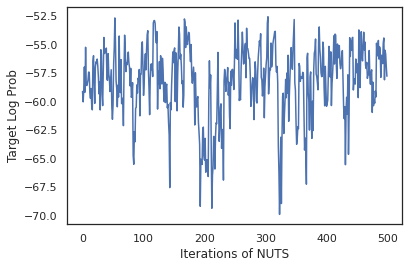
हम से नमूना dist एमसीएमसी के लिए एक प्रारंभिक राज्य निर्माण करने के लिए। फिर हम एक फ़ंक्शन को परिभाषित कर सकते हैं जो एक यादृच्छिक कुंजी और प्रारंभिक स्थिति लेता है, और नो-यू-टर्न-सैंपलर (एनयूटीएस) से 500 नमूने तैयार करता है। ध्यान दें कि हम जैसे JAX परिवर्तनों का उपयोग कर सकते jit XLA का उपयोग कर हमारे पागल नमूना संकलित करने के लिए।
init_key, sample_key = random.split(random.PRNGKey(0))
init_params = tuple(dist.sample(seed=init_key)[:-1])

@jit
def run_chain(key, state):
  kernel = tfp.mcmc.NoUTurnSampler(target_log_prob, 1e-3)
  return tfp.mcmc.sample_chain(500,
      current_state=state,
      kernel=kernel,
      trace_fn=lambda _, results: results.target_log_prob,
      num_burnin_steps=500,
      seed=key)

states, log_probs = run_chain(sample_key, init_params)
plt.figure()
plt.plot(log_probs)
plt.ylabel('Target Log Prob')
plt.xlabel('Iterations of NUTS')
plt.show()
आइए हमारे नमूनों का उपयोग वजन के प्रत्येक सेट की अनुमानित संभावनाओं के औसत से बायेसियन मॉडल औसत (बीएमए) करने के लिए करें।
आइए पहले एक फ़ंक्शन लिखें जो दिए गए मापदंडों के सेट के लिए प्रत्येक वर्ग पर संभावनाओं का उत्पादन करेगा। हम उपयोग कर सकते हैं dist.sample_distributions मॉडल में अंतिम वितरण प्राप्त करने के लिए।
def classifier_probs(params):
  dists, _ = dist.sample_distributions(seed=random.PRNGKey(0),
                                       value=params + (None,))
  return dists[-1].distribution.probs_parameter()
हम कर सकते हैं vmap(classifier_probs) नमूने के समूह के ऊपर हमारे नमूने से प्रत्येक के लिए भविष्यवाणी की वर्ग संभावनाओं को पाने के लिए। फिर हम प्रत्येक नमूने में औसत सटीकता की गणना करते हैं, और बायेसियन मॉडल औसत से सटीकता की गणना करते हैं।
all_probs = jit(vmap(classifier_probs))(states)
print('Average accuracy:', jnp.mean(all_probs.argmax(axis=-1) == labels))
print('BMA accuracy:', jnp.mean(all_probs.mean(axis=0).argmax(axis=-1) == labels))
Average accuracy: 0.96952
BMA accuracy: 0.97999996
ऐसा लगता है कि BMA हमारी त्रुटि दर को लगभग एक तिहाई कम कर देता है!
बुनियादी बातों
TFP JAX पर TF के लिए एक समान एपीआई जहां TF वस्तुओं स्वीकार करने के बजाय की तरह है tf.Tensor है यह JAX एनालॉग स्वीकार करता है। उदाहरण के लिए, जहाँ भी एक tf.Tensor पहले से इनपुट के रूप में इस्तेमाल किया गया था, एपीआई अब एक JAX उम्मीद DeviceArray । इसके बजाय एक लौटने का tf.Tensor , TFP तरीकों वापस आ जाएगी DeviceArray रों। TFP JAX पर भी JAX वस्तुओं की नेस्टेड संरचनाओं, की एक सूची या शब्दकोश की तरह साथ काम करता है DeviceArray रों।
वितरण
TFP के अधिकांश वितरण JAX में उनके TF समकक्षों के समान समानार्थक शब्दों के साथ समर्थित हैं। उन्होंने यह भी रूप में पंजीकृत हैं JAX Pytrees , तो वे इनपुट और JAX-बदल कार्यों के आउटपुट हो सकता है।
बुनियादी वितरण
log_prob वितरण के लिए विधि एक ही काम करता है।
dist = tfd.Normal(0., 1.)
print(dist.log_prob(0.))
-0.9189385
एक वितरण से नमूना स्पष्ट रूप से एक में गुजर आवश्यकता PRNGKey के रूप में (पूर्णांकों की सूची या) seed कीवर्ड तर्क। एक बीज में स्पष्ट रूप से पारित करने में विफल होने पर एक त्रुटि होगी।
tfd.Normal(0., 1.).sample(seed=random.PRNGKey(0))
DeviceArray(-0.20584226, dtype=float32)
वितरण के लिए आकार अर्थ विज्ञान JAX, जहां वितरण प्रत्येक एक होगा में ही रहते हैं event_shape और एक batch_shape और कई नमूने ड्राइंग अतिरिक्त जोड़ देगा sample_shape आयाम।
उदाहरण के लिए, एक tfd.MultivariateNormalDiag वेक्टर मानकों के साथ एक वेक्टर घटना आकार और खाली बैच आकार होगा।
dist = tfd.MultivariateNormalDiag(
    loc=jnp.zeros(5),
    scale_diag=jnp.ones(5)
)
print('Event shape:', dist.event_shape)
print('Batch shape:', dist.batch_shape)
Event shape: (5,)
Batch shape: ()
दूसरी ओर, एक tfd.Normal वैक्टर साथ parameterized एक अदिश घटना आकार और वेक्टर बैच आकार होगा।
dist = tfd.Normal(
    loc=jnp.ones(5),
    scale=jnp.ones(5),
)
print('Event shape:', dist.event_shape)
print('Batch shape:', dist.batch_shape)
Event shape: ()
Batch shape: (5,)
लेने का अर्थ विज्ञान log_prob नमूनों की भी JAX में एक ही काम करता है।
dist =  tfd.Normal(jnp.zeros(5), jnp.ones(5))
s = dist.sample(sample_shape=(10, 2), seed=random.PRNGKey(0))
print(dist.log_prob(s).shape)

dist =  tfd.Independent(tfd.Normal(jnp.zeros(5), jnp.ones(5)), 1)
s = dist.sample(sample_shape=(10, 2), seed=random.PRNGKey(0))
print(dist.log_prob(s).shape)
(10, 2, 5)
(10, 2)
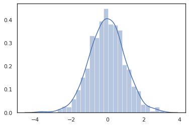
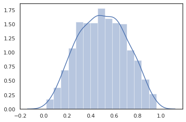
क्योंकि JAX DeviceArray रों NumPy और matplotlib तरह पुस्तकालयों के साथ संगत कर रहे हैं, हम एक साजिश रचने समारोह में सीधे नमूने फ़ीड कर सकते हैं।
sns.distplot(tfd.Normal(0., 1.).sample(1000, seed=random.PRNGKey(0)))
plt.show()
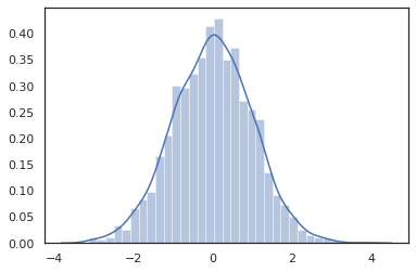
Distribution के तरीकों JAX परिवर्तनों के साथ संगत कर रहे हैं।
sns.distplot(jit(vmap(lambda key: tfd.Normal(0., 1.).sample(seed=key)))(
    random.split(random.PRNGKey(0), 2000)))
plt.show()
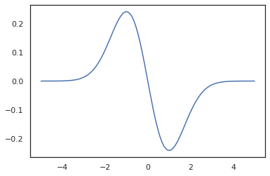
x = jnp.linspace(-5., 5., 100)
plt.plot(x, jit(vmap(grad(tfd.Normal(0., 1.).prob)))(x))
plt.show()
TFP वितरण JAX pytree नोड्स के रूप में पंजीकृत हैं, इसलिए हम आदानों या आउटपुट के रूप में वितरण के साथ काम करता है लिख सकते हैं और का उपयोग कर उन्हें बदलने jit , लेकिन वे अभी तक तर्क के रूप में समर्थित नहीं हैं vmap एड कार्य करता है।
@jit
def random_distribution(key):
  loc_key, scale_key = random.split(key)
  loc, log_scale = random.normal(loc_key), random.normal(scale_key)
  return tfd.Normal(loc, jnp.exp(log_scale))
random_dist = random_distribution(random.PRNGKey(0))
print(random_dist.mean(), random_dist.variance())
0.14389051 0.081832744
रूपांतरित वितरण
बदल वितरण यानी वितरण जिसका नमूने एक के माध्यम से पारित कर रहे हैं Bijector भी बॉक्स से बाहर काम करते हैं (bijectors भी काम करते हैं! नीचे देखें)।
dist = tfd.TransformedDistribution(
    tfd.Normal(0., 1.),
    tfb.Sigmoid()
)
sns.distplot(dist.sample(1000, seed=random.PRNGKey(0)))
plt.show()
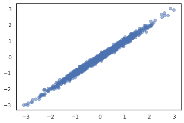
संयुक्त वितरण
TFP प्रदान करता है JointDistribution रों कई यादृच्छिक परिवर्तनीय आने वाले एक वितरण में घटक वितरण के संयोजन सक्षम करने के लिए। वर्तमान में, TFP प्रस्तावों तीन मुख्य वेरिएंट ( JointDistributionSequential , JointDistributionNamed , और JointDistributionCoroutine ) जो सभी के JAX में समर्थित हैं। AutoBatched वेरिएंट भी सभी समर्थित हैं।
dist = tfd.JointDistributionSequential([
  tfd.Normal(0., 1.),
  lambda x: tfd.Normal(x, 1e-1)
])
plt.scatter(*dist.sample(1000, seed=random.PRNGKey(0)), alpha=0.5)
plt.show()
joint = tfd.JointDistributionNamed(dict(
    e=             tfd.Exponential(rate=1.),
    n=             tfd.Normal(loc=0., scale=2.),
    m=lambda n, e: tfd.Normal(loc=n, scale=e),
    x=lambda    m: tfd.Sample(tfd.Bernoulli(logits=m), 12),
))
joint.sample(seed=random.PRNGKey(0))
{'e': DeviceArray(3.376818, dtype=float32),
 'm': DeviceArray(2.5449684, dtype=float32),
 'n': DeviceArray(-0.6027825, dtype=float32),
 'x': DeviceArray([1, 1, 1, 1, 1, 1, 1, 1, 1, 1, 1, 1], dtype=int32)}
Root = tfd.JointDistributionCoroutine.Root
def model():
  e = yield Root(tfd.Exponential(rate=1.))
  n = yield Root(tfd.Normal(loc=0, scale=2.))
  m = yield tfd.Normal(loc=n, scale=e)
  x = yield tfd.Sample(tfd.Bernoulli(logits=m), 12)

joint = tfd.JointDistributionCoroutine(model)

joint.sample(seed=random.PRNGKey(0))
StructTuple(var0=DeviceArray(0.17315261, dtype=float32), var1=DeviceArray(-3.290489, dtype=float32), var2=DeviceArray(-3.1949058, dtype=float32), var3=DeviceArray([0, 0, 0, 0, 0, 0, 0, 0, 0, 0, 0, 0], dtype=int32))
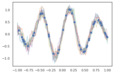
अन्य वितरण
गाऊसी प्रक्रियाएं भी JAX मोड में काम करती हैं!
k1, k2, k3 = random.split(random.PRNGKey(0), 3)
observation_noise_variance = 0.01
f = lambda x: jnp.sin(10*x[..., 0]) * jnp.exp(-x[..., 0]**2)
observation_index_points = random.uniform(
    k1, [50], minval=-1.,maxval= 1.)[..., jnp.newaxis]
observations = f(observation_index_points) + tfd.Normal(
    loc=0., scale=jnp.sqrt(observation_noise_variance)).sample(seed=k2)

index_points = jnp.linspace(-1., 1., 100)[..., jnp.newaxis]

kernel = tfpk.ExponentiatedQuadratic(length_scale=0.1)

gprm = tfd.GaussianProcessRegressionModel(
    kernel=kernel,
    index_points=index_points,
    observation_index_points=observation_index_points,
    observations=observations,
    observation_noise_variance=observation_noise_variance)

samples = gprm.sample(10, seed=k3)
for i in range(10):
  plt.plot(index_points, samples[i], alpha=0.5)
plt.plot(observation_index_points, observations, marker='o', linestyle='')
plt.show()
हिडन मार्कोव मॉडल भी समर्थित हैं।
initial_distribution = tfd.Categorical(probs=[0.8, 0.2])
transition_distribution = tfd.Categorical(probs=[[0.7, 0.3],
                                                 [0.2, 0.8]])

observation_distribution = tfd.Normal(loc=[0., 15.], scale=[5., 10.])

model = tfd.HiddenMarkovModel(
    initial_distribution=initial_distribution,
    transition_distribution=transition_distribution,
    observation_distribution=observation_distribution,
    num_steps=7)

print(model.mean())
print(model.log_prob(jnp.zeros(7)))
print(model.sample(seed=random.PRNGKey(0)))
[3.       6.       7.5      8.249999 8.625001 8.812501 8.90625 ]
/usr/local/lib/python3.6/dist-packages/tensorflow_probability/substrates/jax/distributions/hidden_markov_model.py:483: UserWarning: HiddenMarkovModel.log_prob in TFP versions < 0.12.0 had a bug in which the transition model was applied prior to the initial step. This bug has been fixed. You may observe a slight change in behavior.
  'HiddenMarkovModel.log_prob in TFP versions < 0.12.0 had a bug '
-19.855635
[ 1.3641367  0.505798   1.3626463  3.6541772  2.272286  15.10309
 22.794212 ]
की तरह कुछ वितरण PixelCNN TensorFlow या XLA असंगतियां पर सख्त निर्भरता की वजह से अभी तक समर्थित नहीं हैं।
बिजेक्टर
TFP के अधिकांश बायजेक्टर आज JAX में समर्थित हैं!
tfb.Exp().inverse(1.)
DeviceArray(0., dtype=float32)
bij = tfb.Shift(1.)(tfb.Scale(3.))
print(bij.forward(jnp.ones(5)))
print(bij.inverse(jnp.ones(5)))
[4. 4. 4. 4. 4.]
[0. 0. 0. 0. 0.]
b = tfb.FillScaleTriL(diag_bijector=tfb.Exp(), diag_shift=None)
print(b.forward(x=[0., 0., 0.]))
print(b.inverse(y=[[1., 0], [.5, 2]]))
[[1. 0.]
 [0. 1.]]
[0.6931472 0.5       0.       ]
b = tfb.Chain([tfb.Exp(), tfb.Softplus()])
# or:
# b = tfb.Exp()(tfb.Softplus())
print(b.forward(-jnp.ones(5)))
[1.3678794 1.3678794 1.3678794 1.3678794 1.3678794]
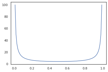
Bijectors तरह JAX परिवर्तनों के साथ संगत कर रहे हैं jit , grad और vmap ।
jit(vmap(tfb.Exp().inverse))(jnp.arange(4.))
DeviceArray([ -inf, 0. , 0.6931472, 1.0986123], dtype=float32)
x = jnp.linspace(0., 1., 100)
plt.plot(x, jit(grad(lambda x: vmap(tfb.Sigmoid().inverse)(x).sum()))(x))
plt.show()
कुछ bijectors, जैसे RealNVP और FFJORD अभी तक समर्थित नहीं हैं।
एमसीएमसी
हम पोर्ट किया है tfp.mcmc रूप में अच्छी तरह JAX के लिए, तो हम Hamiltonian मोंटे कार्लो (एचएमसी) और JAX में नो-यू-टर्न-नमूना (पागल) की तरह एल्गोरिदम चला सकते हैं।
target_log_prob = tfd.MultivariateNormalDiag(jnp.zeros(2), jnp.ones(2)).log_prob
TFP TF पर विपरीत, हम एक पास करना आवश्यक है PRNGKey में sample_chain का उपयोग कर seed कीवर्ड तर्क।
def run_chain(key, state):
kernel = tfp.mcmc.NoUTurnSampler(target_log_prob, 1e-1)
return tfp.mcmc.sample_chain(1000,
current_state=state,
kernel=kernel,
trace_fn=lambda _, results: results.target_log_prob,
seed=key)
states, log_probs = jit(run_chain)(random.PRNGKey(0), jnp.zeros(2))
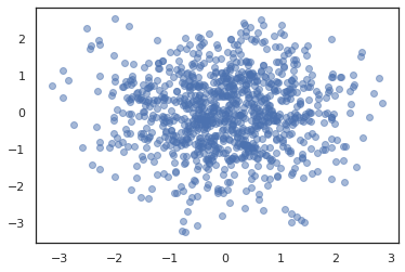
plt.figure()
plt.scatter(*states.T, alpha=0.5)
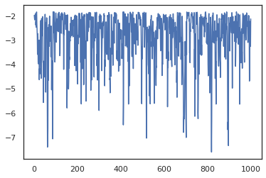
plt.figure()
plt.plot(log_probs)
plt.show()
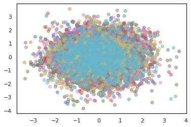
कई चेन चलाने के लिए, हम या तो राज्यों का एक बैच में पारित कर सकते हैं sample_chain या उपयोग vmap (हालांकि हम अभी तक दो दृष्टिकोणों के बीच प्रदर्शन अंतर का पता लगाया नहीं किया है)।
states, log_probs = jit(run_chain)(random.PRNGKey(0), jnp.zeros([10, 2]))
plt.figure()
for i in range(10):
plt.scatter(*states[:, i].T, alpha=0.5)
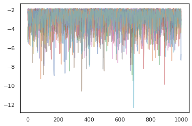
plt.figure()
for i in range(10):
plt.plot(log_probs[:, i], alpha=0.5)
plt.show()
अनुकूलक
जेएक्स पर टीएफपी बीएफजीएस और एल-बीएफजीएस जैसे कुछ महत्वपूर्ण अनुकूलकों का समर्थन करता है। आइए एक साधारण स्केल्ड द्विघात हानि फ़ंक्शन सेट करें।
minimum = jnp.array([1.0, 1.0])  # The center of the quadratic bowl.
scales = jnp.array([2.0, 3.0])  # The scales along the two axes.

# The objective function and the gradient.
def quadratic_loss(x):
  return jnp.sum(scales * jnp.square(x - minimum))

start = jnp.array([0.6, 0.8])  # Starting point for the search.
बीएफजीएस इस नुकसान का न्यूनतम पता लगा सकता है।
optim_results = tfp.optimizer.bfgs_minimize(
    value_and_grad(quadratic_loss), initial_position=start, tolerance=1e-8)

# Check that the search converged
assert(optim_results.converged)
# Check that the argmin is close to the actual value.
np.testing.assert_allclose(optim_results.position, minimum)
# Print out the total number of function evaluations it took. Should be 5.
print("Function evaluations: %d" % optim_results.num_objective_evaluations)
Function evaluations: 5
तो एल-बीएफजीएस कर सकते हैं।
optim_results = tfp.optimizer.lbfgs_minimize(
    value_and_grad(quadratic_loss), initial_position=start, tolerance=1e-8)

# Check that the search converged
assert(optim_results.converged)
# Check that the argmin is close to the actual value.
np.testing.assert_allclose(optim_results.position, minimum)
# Print out the total number of function evaluations it took. Should be 5.
print("Function evaluations: %d" % optim_results.num_objective_evaluations)
Function evaluations: 5
करने के लिए vmap एल BFGS, सेट एक समारोह है कि एक ही प्रारंभिक बिंदु के लिए नुकसान का अनुकूलन अप करते हैं।
def optimize_single(start):
  return tfp.optimizer.lbfgs_minimize(
      value_and_grad(quadratic_loss), initial_position=start, tolerance=1e-8)

all_results = jit(vmap(optimize_single))(
    random.normal(random.PRNGKey(0), (10, 2)))
assert all(all_results.converged)
for i in range(10):
  np.testing.assert_allclose(optim_results.position[i], minimum)
print("Function evaluations: %s" % all_results.num_objective_evaluations)
Function evaluations: [6 6 9 6 6 8 6 8 5 9]
चेतावनियां
TF और JAX के बीच कुछ मूलभूत अंतर हैं, कुछ TFP व्यवहार दो सबस्ट्रेट्स के बीच भिन्न होंगे और सभी कार्यक्षमता समर्थित नहीं हैं। उदाहरण के लिए,
- TFP JAX पर ऐसा कुछ का समर्थन नहीं करता
tf.Variableकुछ भी नहीं के बाद से है जैसे कि यह JAX में मौजूद है। यह भी मतलब है की तरह उपयोगिताओंtfp.util.TransformedVariableया तो समर्थित नहीं हैं। -
tfp.layersपर Keras और अपनी निर्भरता की वजह से अभी तक बैकएंड में समर्थित नहीं है,tf.Variableरों। -
tfp.math.minimizeपर अपनी निर्भरता की वजह से JAX पर TFP में काम नहीं करताtf.Variable। - JAX पर TFP के साथ, टेंसर आकार हमेशा ठोस पूर्णांक मान होते हैं और TF पर TFP की तरह कभी भी अज्ञात/गतिशील नहीं होते हैं।
- छद्म यादृच्छिकता को TF और JAX (परिशिष्ट देखें) में अलग तरह से नियंत्रित किया जाता है।
- में पुस्तकालय
tfp.experimentalJAX सब्सट्रेट में मौजूद गारंटी नहीं है। - TF और JAX के बीच Dtype पदोन्नति नियम भिन्न हैं। जेएक्स पर टीएफपी स्थिरता के लिए आंतरिक रूप से टीएफ के डीटाइप सेमेन्टिक्स का सम्मान करने का प्रयास करता है।
- बिजेक्टर को अभी तक JAX pytrees के रूप में पंजीकृत नहीं किया गया है।
क्या JAX पर TFP में समर्थित है की पूरी सूची देखने के लिए, कृपया को देखें API दस्तावेज़ ।
निष्कर्ष
हमने TFP की बहुत सी विशेषताओं को JAX में पोर्ट किया है और यह देखने के लिए उत्साहित हैं कि हर कोई क्या बनाएगा। कुछ कार्यक्षमता अभी तक समर्थित नहीं है; हम कुछ आप के लिए महत्वपूर्ण नहीं छूटा है अगर (या यदि आप एक बग मिल!) हमें से संपर्क करें - आप ईमेल कर सकते हैं tfprobability@tensorflow.org या पर एक मुद्दा फ़ाइल हमारे Github रेपो ।
परिशिष्ट: JAX . में छद्म यादृच्छिकता
JAX के कूट-यादृच्छिक संख्या पीढ़ी (PRNG) मॉडल राज्यविहीन है। एक स्टेटफुल मॉडल के विपरीत, कोई भी परिवर्तनशील वैश्विक स्थिति नहीं है जो प्रत्येक यादृच्छिक ड्रा के बाद विकसित होती है। JAX के मॉडल में, हम एक PRNG कुंजी है, जो 32-बिट पूर्णांकों की एक जोड़ी की तरह काम करता साथ शुरू करते हैं। हम का उपयोग करके इन कुंजियों का निर्माण कर सकते jax.random.PRNGKey ।
key = random.PRNGKey(0)  # Creates a key with value [0, 0]
print(key)
[0 0]
JAX में रैंडम कार्यों एक महत्वपूर्ण उपभोग करने के लिए निर्धारणात्मक एक यादृच्छिक variate उत्पादन, जिसका अर्थ है कि वे फिर से नहीं किया जाना चाहिए। उदाहरण के लिए, हम उपयोग कर सकते हैं key एक सामान्य रूप से वितरित मूल्य नमूने के लिए है, लेकिन हम उपयोग नहीं करना चाहिए key फिर कहीं और। इसके अलावा, में एक ही मूल्य गुजर random.normal एक ही मूल्य का उत्पादन करेगा।
print(random.normal(key))
-0.20584226
तो हम कभी भी एक ही कुंजी से कई नमूने कैसे खींच सकते हैं? उत्तर कुंजी बंटवारे है। मूल विचार है कि हम एक विभाजित कर सकते हैं है PRNGKey कई में, और नए चाबियों का प्रत्येक अनियमितता के एक स्वतंत्र स्रोत के रूप में इलाज किया जा सकता।
key1, key2 = random.split(key, num=2)
print(key1, key2)
[4146024105 967050713] [2718843009 1272950319]
कुंजी विभाजन नियतात्मक है लेकिन अराजक है, इसलिए प्रत्येक नई कुंजी का उपयोग अब एक अलग यादृच्छिक नमूना बनाने के लिए किया जा सकता है।
print(random.normal(key1), random.normal(key2))
0.14389051 -1.2515389
JAX के नियतात्मक कुंजी बंटवारे मॉडल के बारे में अधिक जानकारी के लिए, इस गाइड ।