| |
 GitHub でソースを表示 GitHub でソースを表示 |
このチュートリアルでは、Isola et al による『Image-to-image translation with conditional adversarial networks』(2017 年)で説明されているように、入力画像から出力画像へのマッピングを学習する pix2pix と呼ばれる条件付き敵対的生成ネットワーク(cGAN)を構築し、トレーニングする方法を説明します。pix2pix はアプリケーションに依存しません。ラベルマップからの写真の合成、モノクロ画像からのカラー写真の生成、Google Maps の写真から航空写真への変換、スケッチ画像から写真への変換など、広範なタスクに適用できます。
この例のネットワークは、プラハにあるチェコ工科大学 の機械知覚センター が提供する CMP Facade Database を使用して、建築物のファサード(正面部)の画像を生成します。この例を手短に紹介できるように、pix2pix の著者が作成したデータセットの事前処理済みのセットを使用します。
pix2pix の cGAN では、入力画像で条件付けを行い、対応する出力画像を生成します。cGANs は『Conditional Generative Adversarial Nets』(2014 年 Mirza and Osindero)おいて初めて言及されました。
ネットワークのアーキテクチャには、以下の項目が含まれます。
- U-Net ベースのアーキテクチャを使用したジェネレータ。
- 畳みこみ PatchGAN 分類器で表現されたディスクリミネータ(pix2pix 論文 で提案)。
単一の V100 GPU で、エポックごとに約 15 秒かかる可能性があります。
以下は、ファサードデータセットを使って 200 エポックトレーニング(8 万ステップ)した後に pix2pix xGAN が生成した出力の例です。
TensorFlow とその他のライブラリをインポートする
import tensorflow as tf

import os
import pathlib
import time
import datetime

from matplotlib import pyplot as plt
from IPython import display
2024-01-11 23:04:41.772344: E external/local_xla/xla/stream_executor/cuda/cuda_dnn.cc:9261] Unable to register cuDNN factory: Attempting to register factory for plugin cuDNN when one has already been registered
2024-01-11 23:04:41.772392: E external/local_xla/xla/stream_executor/cuda/cuda_fft.cc:607] Unable to register cuFFT factory: Attempting to register factory for plugin cuFFT when one has already been registered
2024-01-11 23:04:41.774012: E external/local_xla/xla/stream_executor/cuda/cuda_blas.cc:1515] Unable to register cuBLAS factory: Attempting to register factory for plugin cuBLAS when one has already been registered
データセットを読み込む
CMP Facade データベースのデータをダウンロードします(30 MB)。追加のデータセットはこちら から同じ形式で入手できます。Colab では、ドロップダウンメニューから別のデータセットを選択できます。他のデータベースの一部は非常に大きいことに注意してください(edges2handbags は 8 GB)。
dataset_name = "facades"
_URL = f'http://efrosgans.eecs.berkeley.edu/pix2pix/datasets/{dataset_name}.tar.gz'

path_to_zip = tf.keras.utils.get_file(
    fname=f"{dataset_name}.tar.gz",
    origin=_URL,
    extract=True)

path_to_zip  = pathlib.Path(path_to_zip)

PATH = path_to_zip.parent/dataset_name
Downloading data from http://efrosgans.eecs.berkeley.edu/pix2pix/datasets/facades.tar.gz
30168306/30168306 [==============================] - 19s 1us/step
list(PATH.parent.iterdir())
[PosixPath('/home/kbuilder/.keras/datasets/shakespeare.txt'),
 PosixPath('/home/kbuilder/.keras/datasets/jena_climate_2009_2016.csv.zip'),
 PosixPath('/home/kbuilder/.keras/datasets/cats_and_dogs_filtered'),
 PosixPath('/home/kbuilder/.keras/datasets/Giant Panda'),
 PosixPath('/home/kbuilder/.keras/datasets/spa-eng'),
 PosixPath('/home/kbuilder/.keras/datasets/194px-New_East_River_Bridge_from_Brooklyn_det.4a09796u.jpg'),
 PosixPath('/home/kbuilder/.keras/datasets/cifar-10-batches-py'),
 PosixPath('/home/kbuilder/.keras/datasets/ImageNetLabels.txt'),
 PosixPath('/home/kbuilder/.keras/datasets/320px-Felis_catus-cat_on_snow.jpg'),
 PosixPath('/home/kbuilder/.keras/datasets/iris_training.csv'),
 PosixPath('/home/kbuilder/.keras/datasets/flower_photos.tgz'),
 PosixPath('/home/kbuilder/.keras/datasets/Fireboat'),
 PosixPath('/home/kbuilder/.keras/datasets/iris_test.csv'),
 PosixPath('/home/kbuilder/.keras/datasets/Red_sunflower'),
 PosixPath('/home/kbuilder/.keras/datasets/surf.jpg'),
 PosixPath('/home/kbuilder/.keras/datasets/heart.csv'),
 PosixPath('/home/kbuilder/.keras/datasets/spa-eng.zip'),
 PosixPath('/home/kbuilder/.keras/datasets/fashion-mnist'),
 PosixPath('/home/kbuilder/.keras/datasets/cats_and_dogs.zip'),
 PosixPath('/home/kbuilder/.keras/datasets/mnist.npz'),
 PosixPath('/home/kbuilder/.keras/datasets/HIGGS.csv.gz'),
 PosixPath('/home/kbuilder/.keras/datasets/YellowLabradorLooking_new.jpg'),
 PosixPath('/home/kbuilder/.keras/datasets/cifar-10-batches-py.tar.gz'),
 PosixPath('/home/kbuilder/.keras/datasets/facades.tar.gz'),
 PosixPath('/home/kbuilder/.keras/datasets/jena_climate_2009_2016.csv'),
 PosixPath('/home/kbuilder/.keras/datasets/image.jpg'),
 PosixPath('/home/kbuilder/.keras/datasets/facades'),
 PosixPath('/home/kbuilder/.keras/datasets/flower_photos.tar'),
 PosixPath('/home/kbuilder/.keras/datasets/flower_photos'),
 PosixPath('/home/kbuilder/.keras/datasets/bedroom_hrnet_tutorial.jpg'),
 PosixPath('/home/kbuilder/.keras/datasets/kandinsky5.jpg')]
それぞれの元の画像のサイズは 256 x 512 で、256 x 256 の画像が 2 つ含まれます。
sample_image = tf.io.read_file(str(PATH / 'train/1.jpg'))
sample_image = tf.io.decode_jpeg(sample_image)
print(sample_image.shape)
(256, 512, 3)
plt.figure()
plt.imshow(sample_image)
<matplotlib.image.AxesImage at 0x7f1d23ec9520>
実際の建物のファサードの写真と建築ラベル画像を分離する必要があります。すべてのサイズは 256 x 256 になります。
画像ファイルを読み込んで 2 つの画像テンソルを出力する関数を定義します。
def load(image_file):
  # Read and decode an image file to a uint8 tensor
  image = tf.io.read_file(image_file)
  image = tf.io.decode_jpeg(image)

  # Split each image tensor into two tensors:
  # - one with a real building facade image
  # - one with an architecture label image
  w = tf.shape(image)[1]
  w = w // 2
  input_image = image[:, w:, :]
  real_image = image[:, :w, :]

  # Convert both images to float32 tensors
  input_image = tf.cast(input_image, tf.float32)
  real_image = tf.cast(real_image, tf.float32)

  return input_image, real_image
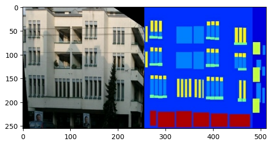
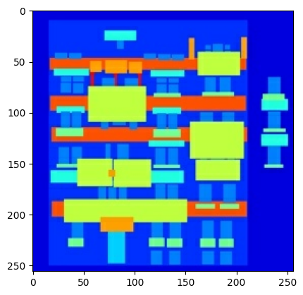
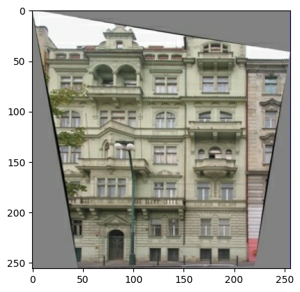
入力(建築ラベル画像)画像と実際の(建物のファサードの写真)画像のサンプルをプロットします。
inp, re = load(str(PATH / 'train/100.jpg'))
# Casting to int for matplotlib to display the images
plt.figure()
plt.imshow(inp / 255.0)
plt.figure()
plt.imshow(re / 255.0)
<matplotlib.image.AxesImage at 0x7f1d1029b9a0>
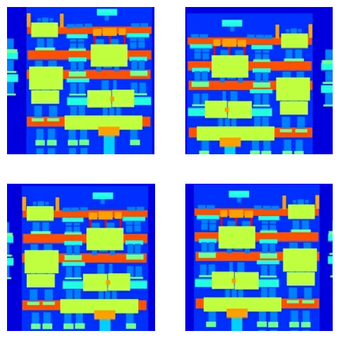
pix2pix 論文 に述べられているように、トレーニングセットを前処理するために、ランダムなジッターとミラーリングを適用する必要があります。
以下を行う関数を定義します。
256 x 256の画像サイズをそれぞれより大きな高さと幅の286 x 286に変更する。- それをランダムに
256 x 256にトリミングする。 - その画像をランダムに横方向(左右)に反転する(ランダムミラーリング)。
- その画像を
[-1, 1]の範囲に正規化する。
# The facade training set consist of 400 images
BUFFER_SIZE = 400
# The batch size of 1 produced better results for the U-Net in the original pix2pix experiment
BATCH_SIZE = 1
# Each image is 256x256 in size
IMG_WIDTH = 256
IMG_HEIGHT = 256
def resize(input_image, real_image, height, width):
  input_image = tf.image.resize(input_image, [height, width],
                                method=tf.image.ResizeMethod.NEAREST_NEIGHBOR)
  real_image = tf.image.resize(real_image, [height, width],
                               method=tf.image.ResizeMethod.NEAREST_NEIGHBOR)

  return input_image, real_image
def random_crop(input_image, real_image):
  stacked_image = tf.stack([input_image, real_image], axis=0)
  cropped_image = tf.image.random_crop(
      stacked_image, size=[2, IMG_HEIGHT, IMG_WIDTH, 3])

  return cropped_image[0], cropped_image[1]
# Normalizing the images to [-1, 1]
def normalize(input_image, real_image):
  input_image = (input_image / 127.5) - 1
  real_image = (real_image / 127.5) - 1

  return input_image, real_image
@tf.function()
def random_jitter(input_image, real_image):
  # Resizing to 286x286
  input_image, real_image = resize(input_image, real_image, 286, 286)

  # Random cropping back to 256x256
  input_image, real_image = random_crop(input_image, real_image)

  if tf.random.uniform(()) > 0.5:
    # Random mirroring
    input_image = tf.image.flip_left_right(input_image)
    real_image = tf.image.flip_left_right(real_image)

  return input_image, real_image
前処理された一部の出力を検査することができます。
plt.figure(figsize=(6, 6))
for i in range(4):
  rj_inp, rj_re = random_jitter(inp, re)
  plt.subplot(2, 2, i + 1)
  plt.imshow(rj_inp / 255.0)
  plt.axis('off')
plt.show()
読み込みと前処理がうまく機能することを確認したら、トレーニングセットとテストセットを読み込んで前処理するヘルパー関数を 2 つ定義しましょう。
def load_image_train(image_file):
  input_image, real_image = load(image_file)
  input_image, real_image = random_jitter(input_image, real_image)
  input_image, real_image = normalize(input_image, real_image)

  return input_image, real_image
def load_image_test(image_file):
  input_image, real_image = load(image_file)
  input_image, real_image = resize(input_image, real_image,
                                   IMG_HEIGHT, IMG_WIDTH)
  input_image, real_image = normalize(input_image, real_image)

  return input_image, real_image
tf.data を使用して入力パイプラインを構築する
train_dataset = tf.data.Dataset.list_files(str(PATH / 'train/*.jpg'))
train_dataset = train_dataset.map(load_image_train,
                                  num_parallel_calls=tf.data.AUTOTUNE)
train_dataset = train_dataset.shuffle(BUFFER_SIZE)
train_dataset = train_dataset.batch(BATCH_SIZE)
try:
  test_dataset = tf.data.Dataset.list_files(str(PATH / 'test/*.jpg'))
except tf.errors.InvalidArgumentError:
  test_dataset = tf.data.Dataset.list_files(str(PATH / 'val/*.jpg'))
test_dataset = test_dataset.map(load_image_test)
test_dataset = test_dataset.batch(BATCH_SIZE)
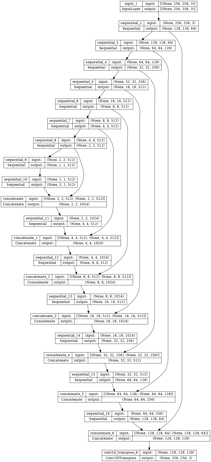
ジェネレータを構築する
pix2pix cGAN のジェネレータは、調整済みの U-Net です。U-Net は、エンコーダ(ダウンサンプラー)とデコーダ(アップサンプラー)で構成されています。(これについては、画像のセグメンテーションチュートリアルと U-Net プロジェクトのウェブサイト をご覧ください。)
- エンコーダの各ブロック: 畳み込み -> バッチ正規化 -> Leaky ReLU
- デコーダの各ブロック: 転置畳み込み -> バッチ正規化 -> ドロップアウト(最初の 3 つのブロックに適用) -> ReLU
- エンコーダとデコーダ間にはスキップ接続があります(U-Net と同じ)。
ダウンサンプラー(エンコーダ)を定義します。
OUTPUT_CHANNELS = 3
def downsample(filters, size, apply_batchnorm=True):
  initializer = tf.random_normal_initializer(0., 0.02)

  result = tf.keras.Sequential()
  result.add(
      tf.keras.layers.Conv2D(filters, size, strides=2, padding='same',
                             kernel_initializer=initializer, use_bias=False))

  if apply_batchnorm:
    result.add(tf.keras.layers.BatchNormalization())

  result.add(tf.keras.layers.LeakyReLU())

  return result
down_model = downsample(3, 4)
down_result = down_model(tf.expand_dims(inp, 0))
print (down_result.shape)
(1, 128, 128, 3)
アップサンプラー(デコーダ)を定義します。
def upsample(filters, size, apply_dropout=False):
  initializer = tf.random_normal_initializer(0., 0.02)

  result = tf.keras.Sequential()
  result.add(
    tf.keras.layers.Conv2DTranspose(filters, size, strides=2,
                                    padding='same',
                                    kernel_initializer=initializer,
                                    use_bias=False))

  result.add(tf.keras.layers.BatchNormalization())

  if apply_dropout:
      result.add(tf.keras.layers.Dropout(0.5))

  result.add(tf.keras.layers.ReLU())

  return result
up_model = upsample(3, 4)
up_result = up_model(down_result)
print (up_result.shape)
(1, 256, 256, 3)
ダウンサンプラーとアップサンプラーを使用してジェネレータを定義します。
def Generator():
  inputs = tf.keras.layers.Input(shape=[256, 256, 3])

  down_stack = [
    downsample(64, 4, apply_batchnorm=False),  # (batch_size, 128, 128, 64)
    downsample(128, 4),  # (batch_size, 64, 64, 128)
    downsample(256, 4),  # (batch_size, 32, 32, 256)
    downsample(512, 4),  # (batch_size, 16, 16, 512)
    downsample(512, 4),  # (batch_size, 8, 8, 512)
    downsample(512, 4),  # (batch_size, 4, 4, 512)
    downsample(512, 4),  # (batch_size, 2, 2, 512)
    downsample(512, 4),  # (batch_size, 1, 1, 512)
  ]

  up_stack = [
    upsample(512, 4, apply_dropout=True),  # (batch_size, 2, 2, 1024)
    upsample(512, 4, apply_dropout=True),  # (batch_size, 4, 4, 1024)
    upsample(512, 4, apply_dropout=True),  # (batch_size, 8, 8, 1024)
    upsample(512, 4),  # (batch_size, 16, 16, 1024)
    upsample(256, 4),  # (batch_size, 32, 32, 512)
    upsample(128, 4),  # (batch_size, 64, 64, 256)
    upsample(64, 4),  # (batch_size, 128, 128, 128)
  ]

  initializer = tf.random_normal_initializer(0., 0.02)
  last = tf.keras.layers.Conv2DTranspose(OUTPUT_CHANNELS, 4,
                                         strides=2,
                                         padding='same',
                                         kernel_initializer=initializer,
                                         activation='tanh')  # (batch_size, 256, 256, 3)

  x = inputs

  # Downsampling through the model
  skips = []
  for down in down_stack:
    x = down(x)
    skips.append(x)

  skips = reversed(skips[:-1])

  # Upsampling and establishing the skip connections
  for up, skip in zip(up_stack, skips):
    x = up(x)
    x = tf.keras.layers.Concatenate()([x, skip])

  x = last(x)

  return tf.keras.Model(inputs=inputs, outputs=x)
ジェネレータモデルアーキテクチャを可視化します。
generator = Generator()
tf.keras.utils.plot_model(generator, show_shapes=True, dpi=64)
ジェネレータをテストします。
gen_output = generator(inp[tf.newaxis, ...], training=False)
plt.imshow(gen_output[0, ...])
Clipping input data to the valid range for imshow with RGB data ([0..1] for floats or [0..255] for integers).
<matplotlib.image.AxesImage at 0x7f1ccc0d6040>
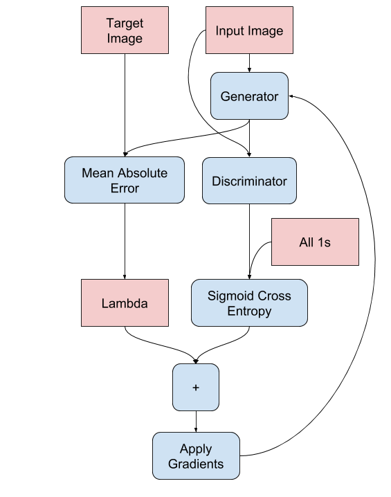
ジェネレータ損失を定義する
pix2pix 論文 によると、GAN はデータに適応する損失を学習するのに対し、cGAN はネットワーク出力とターゲット画像とは異なる可能性のある構造にペナルティを与える構造化損失を学習します。
- ジェネレータ損失は、生成された画像と 1 の配列のシグモイド交差エントロピー損失です。
- pix2pix 論文には、生成された画像とターゲット画像間の MAE(平均絶対誤差)である L1 損失も言及されています。
- これにより、生成された画像は、構造的にターゲット画像に似るようになります。
- 合計ジェネレータ損失の計算式は、
gan_loss + LAMBDA * l1_lossで、LAMBDA = 100です。この値は論文の執筆者が決定したものです。
LAMBDA = 100
loss_object = tf.keras.losses.BinaryCrossentropy(from_logits=True)
def generator_loss(disc_generated_output, gen_output, target):
  gan_loss = loss_object(tf.ones_like(disc_generated_output), disc_generated_output)

  # Mean absolute error
  l1_loss = tf.reduce_mean(tf.abs(target - gen_output))

  total_gen_loss = gan_loss + (LAMBDA * l1_loss)

  return total_gen_loss, gan_loss, l1_loss
以下に、ジェネレータのトレーニング手順を示します。
ディスクリミネータを構築する
pix2pix cGAN のディスクリミネータは、畳み込み PatchGAN 分類器です。pix2pix 論文{:.external} によると、これは、各画像のパッチが本物であるか偽物であるかの分類を試みます。
- ディスクリミネータの各ブロック: 畳み込み -> バッチ正規化 -> Leaky ReLU
- 最後のレイヤーの後の出力の形状:
(batch_size, 30, 30, 1) - 出力の各
30 x 30の画像パッチは入力画像の70 x 70の部分を分類します。 - ディスクリミネータは 2 つの入力を受け取ります。
- 入力画像とターゲット画像。本物として分類する画像です。
- 入力画像と生成された画像(ジェネレータの出力)。偽物として分類する画像です。
tf.concat([inp, tar], axis=-1)を使用して、これら 2 つの入力を連結します。
ディスクリミネータを定義しましょう。
def Discriminator():
  initializer = tf.random_normal_initializer(0., 0.02)

  inp = tf.keras.layers.Input(shape=[256, 256, 3], name='input_image')
  tar = tf.keras.layers.Input(shape=[256, 256, 3], name='target_image')

  x = tf.keras.layers.concatenate([inp, tar])  # (batch_size, 256, 256, channels*2)

  down1 = downsample(64, 4, False)(x)  # (batch_size, 128, 128, 64)
  down2 = downsample(128, 4)(down1)  # (batch_size, 64, 64, 128)
  down3 = downsample(256, 4)(down2)  # (batch_size, 32, 32, 256)

  zero_pad1 = tf.keras.layers.ZeroPadding2D()(down3)  # (batch_size, 34, 34, 256)
  conv = tf.keras.layers.Conv2D(512, 4, strides=1,
                                kernel_initializer=initializer,
                                use_bias=False)(zero_pad1)  # (batch_size, 31, 31, 512)

  batchnorm1 = tf.keras.layers.BatchNormalization()(conv)

  leaky_relu = tf.keras.layers.LeakyReLU()(batchnorm1)

  zero_pad2 = tf.keras.layers.ZeroPadding2D()(leaky_relu)  # (batch_size, 33, 33, 512)

  last = tf.keras.layers.Conv2D(1, 4, strides=1,
                                kernel_initializer=initializer)(zero_pad2)  # (batch_size, 30, 30, 1)

  return tf.keras.Model(inputs=[inp, tar], outputs=last)
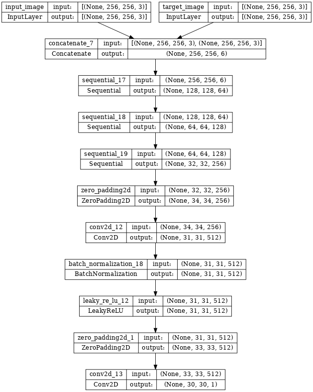
ディスクリミネータモデルアーキテクチャを可視化します。
discriminator = Discriminator()
tf.keras.utils.plot_model(discriminator, show_shapes=True, dpi=64)
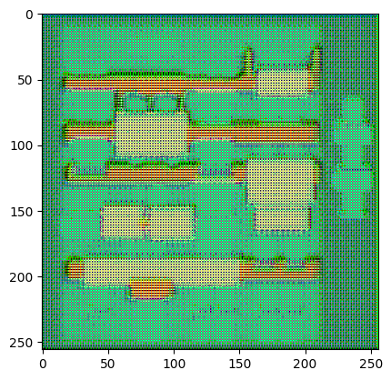
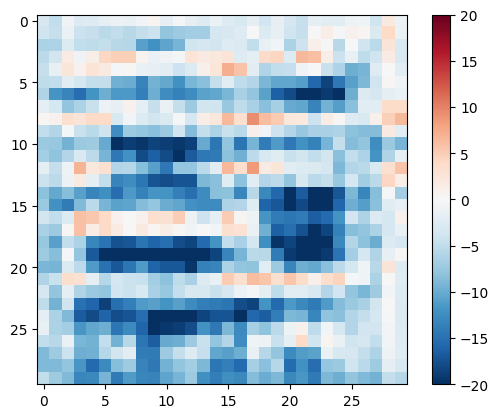
ディスクリミネータをテストします。
disc_out = discriminator([inp[tf.newaxis, ...], gen_output], training=False)
plt.imshow(disc_out[0, ..., -1], vmin=-20, vmax=20, cmap='RdBu_r')
plt.colorbar()
<matplotlib.colorbar.Colorbar at 0x7f1ccc0e9f10>
ディスクリミネータ損失を定義する
discriminator_loss関数は、本物の画像と生成された画像の 2 つの入力を取ります。real_lossは 本物の画像と 1 の配列(本物の画像であるため)のシグモイド交差エントロピー損失です。generated_lossは、生成された画像と 0 の配列(偽物の画像であるため)のシグモイド交差エントロピー損失です。total_lossは、real_lossとgenerated_lossの和です。
def discriminator_loss(disc_real_output, disc_generated_output):
  real_loss = loss_object(tf.ones_like(disc_real_output), disc_real_output)

  generated_loss = loss_object(tf.zeros_like(disc_generated_output), disc_generated_output)

  total_disc_loss = real_loss + generated_loss

  return total_disc_loss
以下に、ディスクリミネータのトレーニング手順を示します。
このアーキテクチャとハイパーパラメータについては、pix2pix 論文 をご覧ください。
オプティマイザとチェックポイントセーバーを定義する
generator_optimizer = tf.keras.optimizers.Adam(2e-4, beta_1=0.5)
discriminator_optimizer = tf.keras.optimizers.Adam(2e-4, beta_1=0.5)
checkpoint_dir = './training_checkpoints'
checkpoint_prefix = os.path.join(checkpoint_dir, "ckpt")
checkpoint = tf.train.Checkpoint(generator_optimizer=generator_optimizer,
                                 discriminator_optimizer=discriminator_optimizer,
                                 generator=generator,
                                 discriminator=discriminator)
画像を生成する
トレーニング中に画像を描画する関数を記述します。
- テストセットの画像をジェネレータに渡します。
- ジェネレータは入力画像を出力に変換します。
- 最後に、予測をプロットすると、出来上がり!
注意: training=True は、テストデータセットでモデルを実行中にバッチ統計を行うために、ここに意図的に指定されています。training=False を使用した場合、トレーニングデータセットから学習した蓄積された統計が取得されます(ここでは使用したくないデータです)。
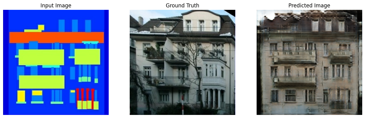
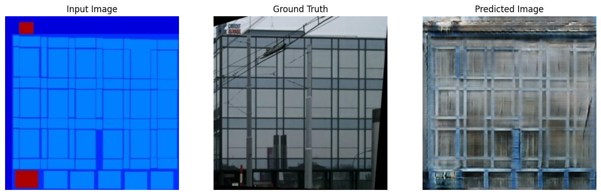
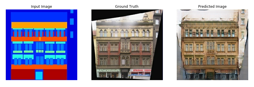
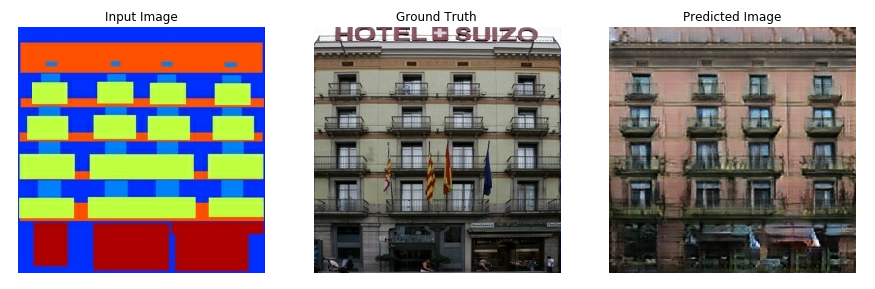
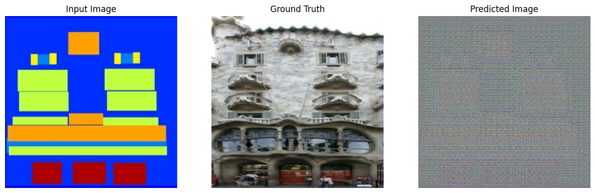
def generate_images(model, test_input, tar):
  prediction = model(test_input, training=True)
  plt.figure(figsize=(15, 15))

  display_list = [test_input[0], tar[0], prediction[0]]
  title = ['Input Image', 'Ground Truth', 'Predicted Image']

  for i in range(3):
    plt.subplot(1, 3, i+1)
    plt.title(title[i])
    # Getting the pixel values in the [0, 1] range to plot.
    plt.imshow(display_list[i] * 0.5 + 0.5)
    plt.axis('off')
  plt.show()
関数をテストします。
for example_input, example_target in test_dataset.take(1):
  generate_images(generator, example_input, example_target)
トレーニング
- 各サンプルについて、入力は出力を生成します。
- ディスクリミネータは input_image と生成された画像を最初の入力として受け取ります。2 番目の入力は input_image と target_image です。
- 次に、ジェネレータとディスクリミネータの損失を計算します。
- さらに、ジェネレータとディスクリミネータの変数(入力)の両方に関して損失の勾配を計算し、これらをオプティマイザに適用します。
- 最後に、損失を TensorBoard にログします。
log_dir="logs/"

summary_writer = tf.summary.create_file_writer(
  log_dir + "fit/" + datetime.datetime.now().strftime("%Y%m%d-%H%M%S"))
@tf.function
def train_step(input_image, target, step):
  with tf.GradientTape() as gen_tape, tf.GradientTape() as disc_tape:
    gen_output = generator(input_image, training=True)

    disc_real_output = discriminator([input_image, target], training=True)
    disc_generated_output = discriminator([input_image, gen_output], training=True)

    gen_total_loss, gen_gan_loss, gen_l1_loss = generator_loss(disc_generated_output, gen_output, target)
    disc_loss = discriminator_loss(disc_real_output, disc_generated_output)

  generator_gradients = gen_tape.gradient(gen_total_loss,
                                          generator.trainable_variables)
  discriminator_gradients = disc_tape.gradient(disc_loss,
                                               discriminator.trainable_variables)

  generator_optimizer.apply_gradients(zip(generator_gradients,
                                          generator.trainable_variables))
  discriminator_optimizer.apply_gradients(zip(discriminator_gradients,
                                              discriminator.trainable_variables))

  with summary_writer.as_default():
    tf.summary.scalar('gen_total_loss', gen_total_loss, step=step//1000)
    tf.summary.scalar('gen_gan_loss', gen_gan_loss, step=step//1000)
    tf.summary.scalar('gen_l1_loss', gen_l1_loss, step=step//1000)
    tf.summary.scalar('disc_loss', disc_loss, step=step//1000)
実際のトレーニングループ。このチュートリアルは 2 つ以上のデータセットを実行でき、データセットのサイズは非常に大きく異なるため、トレーニングループはエポックではなくステップで動作するようにセットアップされています。
- ステップの回数をイテレートします。
- 10 ステップごとにドット(
.)を出力します。 - 1000 ステップごとに、表示を消去し、
generate_imagesを実行して進行状況を示します。 - 5000 ステップごとに、チェックポイントを保存します。
def fit(train_ds, test_ds, steps):
  example_input, example_target = next(iter(test_ds.take(1)))
  start = time.time()

  for step, (input_image, target) in train_ds.repeat().take(steps).enumerate():
    if (step) % 1000 == 0:
      display.clear_output(wait=True)

      if step != 0:
        print(f'Time taken for 1000 steps: {time.time()-start:.2f} sec\n')

      start = time.time()

      generate_images(generator, example_input, example_target)
      print(f"Step: {step//1000}k")

    train_step(input_image, target, step)

    # Training step
    if (step+1) % 10 == 0:
      print('.', end='', flush=True)


    # Save (checkpoint) the model every 5k steps
    if (step + 1) % 5000 == 0:
      checkpoint.save(file_prefix=checkpoint_prefix)
このトレーニングループは、TensorBoard に表示してトレーニングの進行状況を監視できるようにログを保存します。
ローカルマシンで作業する場合は、別の TensorBoard プロセスが起動します。ノートブックで作業する場合は、トレーニングを起動する前にビューアーを起動して、TensorBoard で監視します。
TensorFlow ビューアーを起動します(残念ながら、tensorflow.org では表示されません):
%load_ext tensorboard
%tensorboard --logdir {log_dir}
TensorBoard.dev で、このノートブックの前回の実行結果を閲覧できます。
最後に、トレーニングループを実行します。
fit(train_dataset, test_dataset, steps=40000)
Time taken for 1000 steps: 93.30 sec
Step: 39k
....................................................................................................
GAN(または pix2pix のような cGAN)をトレーニングする場合、ログの解釈は、単純な分類または回帰モデルよりも明確ではありません。以下の項目に注目してください。
- ジェネレータまたはディスクリミネータのいずれのモデルにも "won" がないことを確認してください。
gen_gan_lossまたはdisc_lossのいずれかが非常に低い場合、そのモデルがもう片方のモデルを上回っていることを示しているため、組み合わされたモデルを正しくトレーニングできていないことになります。 - 値
log(2) = 0.69は、これらの損失に適した基準点です。パープレキシティ(予測性能)が 2 であるということは、ディスクリミネータが、平均して 2 つのオプションについて等しく不確実であることを表します。 disc_lossについては、値が0.69を下回る場合、ディスクリミネータは、本物の画像と生成された画像を組み合わせたセットにおいて、ランダムよりも優れていることを示します。gen_gan_lossについては、値が0.69を下回る場合、ジェネレータがディスクリミネータを騙すことにおいて、ランダムよりも優れていることを示します。- トレーニングが進行するにつれ、
gen_l1_lossは下降します。
最後のチェックポイントを復元してネットワークをテストする
ls {checkpoint_dir}checkpoint ckpt-5.data-00000-of-00001 ckpt-1.data-00000-of-00001 ckpt-5.index ckpt-1.index ckpt-6.data-00000-of-00001 ckpt-2.data-00000-of-00001 ckpt-6.index ckpt-2.index ckpt-7.data-00000-of-00001 ckpt-3.data-00000-of-00001 ckpt-7.index ckpt-3.index ckpt-8.data-00000-of-00001 ckpt-4.data-00000-of-00001 ckpt-8.index ckpt-4.index
# Restoring the latest checkpoint in checkpoint_dir
checkpoint.restore(tf.train.latest_checkpoint(checkpoint_dir))
<tensorflow.python.checkpoint.checkpoint.CheckpointLoadStatus at 0x7f1c4042ed30>
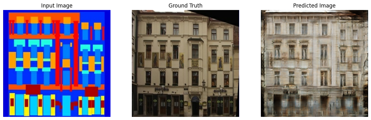
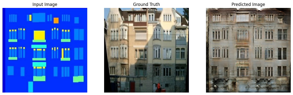
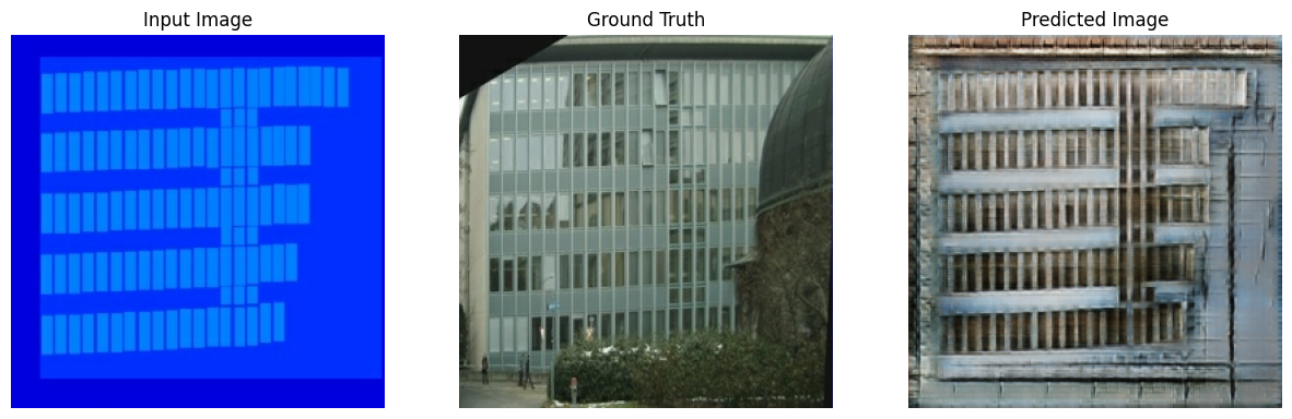
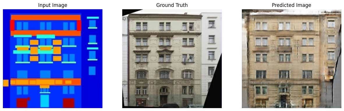
テストセットを使用して画像を生成する
# Run the trained model on a few examples from the test set
for inp, tar in test_dataset.take(5):
  generate_images(generator, inp, tar)