
| |
|
 GitHub でソースを表示 GitHub でソースを表示 |
このチュートリアルでは、修正した U-Net を使用した画像セグメンテーションのタスクに焦点を当てます。
画像セグメンテーションとは
画像分類タスクでは、ネットワークが各入力画像にラベル(またはクラス)を割り当てますが、そのオブジェクトの形状やどのピクセルがどのオブジェクトに属しているかなどを知りたい場合はどうすればよいでしょうか。この場合、画像のピクセルごとにクラスを割り当てる必要があります。このタスクはセグメンテーションとして知られています。セグメンテーションモデルは、画像に関してはるかに詳細な情報を返します。画像セグメンテーションには、医用イメージング、自動走行車、衛星撮像など、数多くの用途があります。
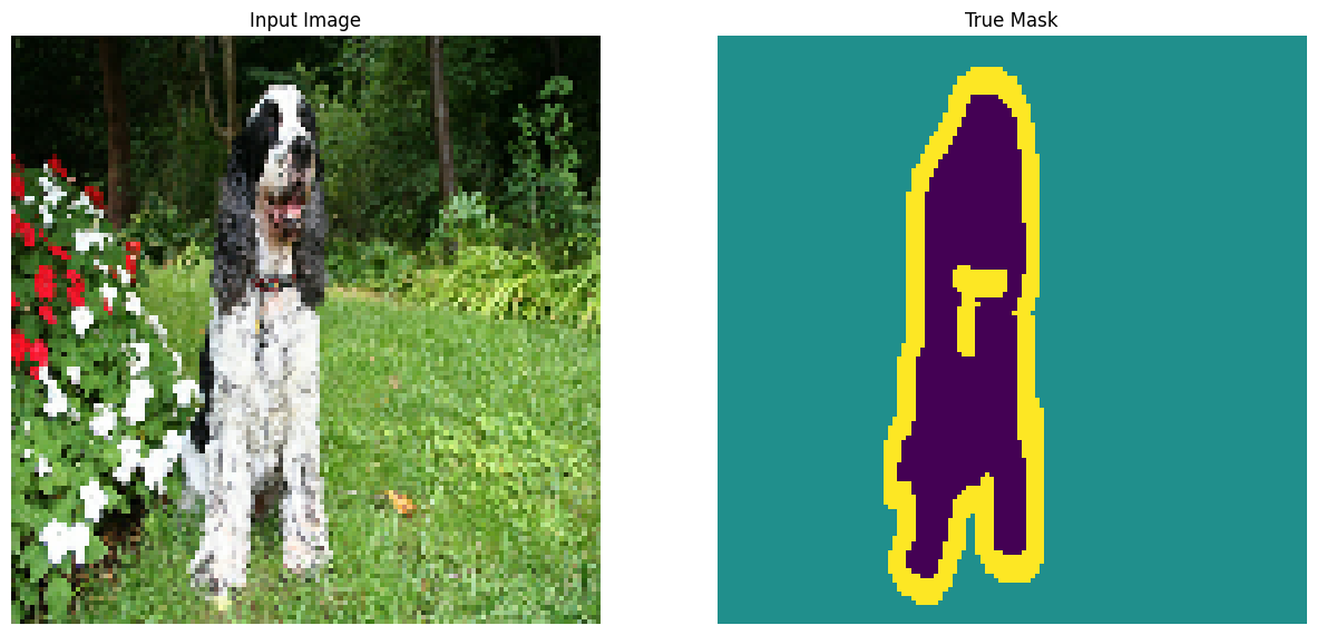
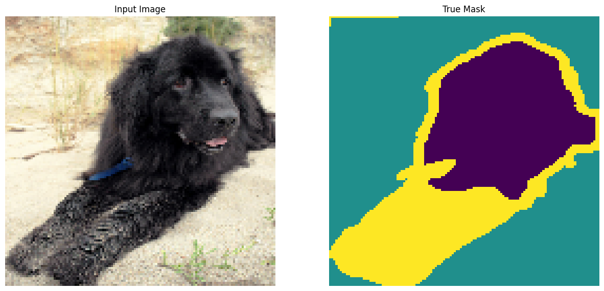
このチュートリアルでは Oxford-IIIT Pet Dataset(Parkhi et al)を使用します。データセットには、37 種のペット品種と、品種当たり 200 枚の画像(train と test split で約 100 枚ずつ)が含まれます。それぞれの画像には対応するラベルとピクセル方向のマスクが含まれます。マスクは各ピクセルのクラスラベルです。各ピクセルには、次のいずれかのカテゴリが指定されます。
- クラス 1 : ペットに属するピクセル。
- クラス 2 : ペットと境界のピクセル。
- クラス 3: 上記のいずれにも該当しない、または周囲のピクセル。
pip install git+https://github.com/tensorflow/examples.gitimport tensorflow as tf
import tensorflow_datasets as tfds
2024-01-11 22:13:08.059220: E external/local_xla/xla/stream_executor/cuda/cuda_dnn.cc:9261] Unable to register cuDNN factory: Attempting to register factory for plugin cuDNN when one has already been registered
2024-01-11 22:13:08.059274: E external/local_xla/xla/stream_executor/cuda/cuda_fft.cc:607] Unable to register cuFFT factory: Attempting to register factory for plugin cuFFT when one has already been registered
2024-01-11 22:13:08.060838: E external/local_xla/xla/stream_executor/cuda/cuda_blas.cc:1515] Unable to register cuBLAS factory: Attempting to register factory for plugin cuBLAS when one has already been registered
from tensorflow_examples.models.pix2pix import pix2pix

from IPython.display import clear_output
import matplotlib.pyplot as plt
Oxford-IIIT ペットデータセットをダウンロードする
データセットは TensorFlow Datasets から入手できます。セグメンテーションマスクはバージョン 3 以上に含まれています。
dataset, info = tfds.load('oxford_iiit_pet:3.*.*', with_info=True)
また、画像の色値は [0,1] の範囲に正規化されています。最後に、上記で説明したとおり、セグメンテーションのマスクは {1, 2, 3} のいずれかでラベル付けされています。便宜上、セグメンテーションマスクから 1 を減算して、ラベルを {0, 1, 2} としましょう。
def normalize(input_image, input_mask):
  input_image = tf.cast(input_image, tf.float32) / 255.0
  input_mask -= 1
  return input_image, input_mask
def load_image(datapoint):
  input_image = tf.image.resize(datapoint['image'], (128, 128))
  input_mask = tf.image.resize(
    datapoint['segmentation_mask'],
    (128, 128),
    method = tf.image.ResizeMethod.NEAREST_NEIGHBOR,
  )

  input_image, input_mask = normalize(input_image, input_mask)

  return input_image, input_mask
データセットにはすでに必要となる training と test split が含まれているため、そのまま同じ split を使用します。
TRAIN_LENGTH = info.splits['train'].num_examples
BATCH_SIZE = 64
BUFFER_SIZE = 1000
STEPS_PER_EPOCH = TRAIN_LENGTH // BATCH_SIZE
train_images = dataset['train'].map(load_image, num_parallel_calls=tf.data.AUTOTUNE)
test_images = dataset['test'].map(load_image, num_parallel_calls=tf.data.AUTOTUNE)
次のクラスは、画像をランダムにフリップする単純な拡張を実行します。詳細は、画像のデータ拡張チュートリアルをご覧ください。
class Augment(tf.keras.layers.Layer):
  def __init__(self, seed=42):
    super().__init__()
    # both use the same seed, so they'll make the same random changes.
    self.augment_inputs = tf.keras.layers.RandomFlip(mode="horizontal", seed=seed)
    self.augment_labels = tf.keras.layers.RandomFlip(mode="horizontal", seed=seed)

  def call(self, inputs, labels):
    inputs = self.augment_inputs(inputs)
    labels = self.augment_labels(labels)
    return inputs, labels
入力パイプラインを構築し、入力をバッチ処理した後に拡張を適用します。
train_batches = (
    train_images
    .cache()
    .shuffle(BUFFER_SIZE)
    .batch(BATCH_SIZE)
    .repeat()
    .map(Augment())
    .prefetch(buffer_size=tf.data.AUTOTUNE))

test_batches = test_images.batch(BATCH_SIZE)
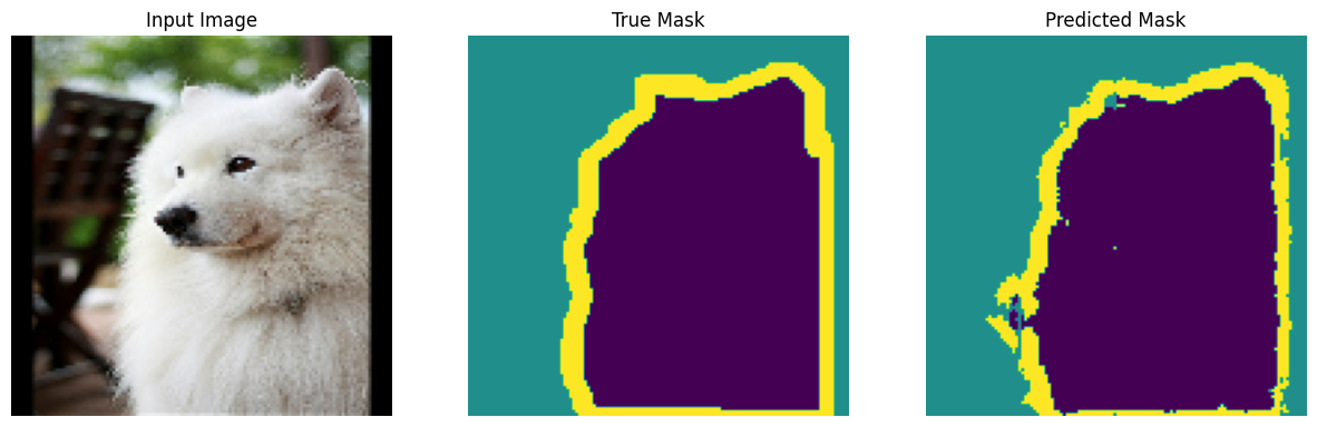
データセットの画像サンプルと対応するマスクを可視化しましょう。
def display(display_list):
  plt.figure(figsize=(15, 15))

  title = ['Input Image', 'True Mask', 'Predicted Mask']

  for i in range(len(display_list)):
    plt.subplot(1, len(display_list), i+1)
    plt.title(title[i])
    plt.imshow(tf.keras.utils.array_to_img(display_list[i]))
    plt.axis('off')
  plt.show()
for images, masks in train_batches.take(2):
  sample_image, sample_mask = images[0], masks[0]
  display([sample_image, sample_mask])
Corrupt JPEG data: 240 extraneous bytes before marker 0xd9
Corrupt JPEG data: premature end of data segment
2024-01-11 22:13:16.387628: W tensorflow/core/kernels/data/cache_dataset_ops.cc:858] The calling iterator did not fully read the dataset being cached. In order to avoid unexpected truncation of the dataset, the partially cached contents of the dataset will be discarded. This can happen if you have an input pipeline similar to `dataset.cache().take(k).repeat()`. You should use `dataset.take(k).cache().repeat()` instead.
モデルを定義する
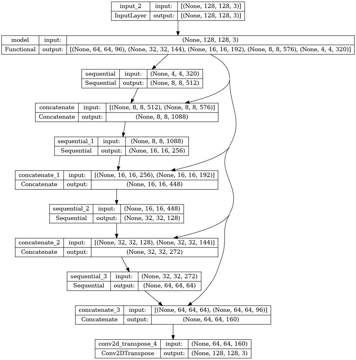
ここで使用されるモデルは変更された U-Net です。U-Net には、エンコーダ(ダウンサンプラー)とデコーダ(アップサンプラー)が含まれます。強力な特徴量を理解してトレーニング可能なパラメータ数を減らすため、MobileNetV2 というトレーニング済みモデルをエンコーダとして使用します。デコーダについてはアップサンプルブロックを使用しますが、これは TensorFlow Examples リポジトリの pix2pix の例に実装済みです。(ノートブックの pix2pix: 条件付き GAN を使用して画像から画像に変換するチュートリアルをご覧ください。)
前述のとおり、エンコーダは事前トレーニング済みの MobileNetV2 モデルです。tf.keras.applications からそのモデルを使用します。エンコーダはモデル内の中間レイヤーからの特定の出力で構成されています。トレーニングプロセス中にエンコーダはトレーニングされないので注意してください。
base_model = tf.keras.applications.MobileNetV2(input_shape=[128, 128, 3], include_top=False)

# Use the activations of these layers
layer_names = [
    'block_1_expand_relu',   # 64x64
    'block_3_expand_relu',   # 32x32
    'block_6_expand_relu',   # 16x16
    'block_13_expand_relu',  # 8x8
    'block_16_project',      # 4x4
]
base_model_outputs = [base_model.get_layer(name).output for name in layer_names]

# Create the feature extraction model
down_stack = tf.keras.Model(inputs=base_model.input, outputs=base_model_outputs)

down_stack.trainable = False
Downloading data from https://storage.googleapis.com/tensorflow/keras-applications/mobilenet_v2/mobilenet_v2_weights_tf_dim_ordering_tf_kernels_1.0_128_no_top.h5
9406464/9406464 [==============================] - 0s 0us/step
デコーダおよびアップサンプラは、単に TensorFlow の 例に実装されている一連のアップサンプラブロックに過ぎません。
up_stack = [
    pix2pix.upsample(512, 3),  # 4x4 -> 8x8
    pix2pix.upsample(256, 3),  # 8x8 -> 16x16
    pix2pix.upsample(128, 3),  # 16x16 -> 32x32
    pix2pix.upsample(64, 3),   # 32x32 -> 64x64
]
def unet_model(output_channels:int):
  inputs = tf.keras.layers.Input(shape=[128, 128, 3])

  # Downsampling through the model
  skips = down_stack(inputs)
  x = skips[-1]
  skips = reversed(skips[:-1])

  # Upsampling and establishing the skip connections
  for up, skip in zip(up_stack, skips):
    x = up(x)
    concat = tf.keras.layers.Concatenate()
    x = concat([x, skip])

  # This is the last layer of the model
  last = tf.keras.layers.Conv2DTranspose(
      filters=output_channels, kernel_size=3, strides=2,
      padding='same')  #64x64 -> 128x128

  x = last(x)

  return tf.keras.Model(inputs=inputs, outputs=x)
最後のレイヤーのフィルタ数は output_channels の数に設定されています。これはクラス当たり 1 つの出力チャンネルとなります。
モデルをトレーニングする
では、後は、モデルををコンパイルしてトレーニングするだけです。
これはマルチクラスの分類問題であり、ラベルがクラスごとのピクセルのスコアのベクトルではなくスカラー整数であるため、tf.keras.losses.SparseCategoricalCrossentropy 損失関数を使用して、from_logits を True に設定します。
推論を実行すると、ピクセルに割り当てられたラベルが最も高い値を持つチャンネルです。これは、create_mask 関数の作用です。
OUTPUT_CLASSES = 3

model = unet_model(output_channels=OUTPUT_CLASSES)
model.compile(optimizer='adam',
              loss=tf.keras.losses.SparseCategoricalCrossentropy(from_logits=True),
              metrics=['accuracy'])
結果のモデルアーキテクチャをプロットしてみましょう。
tf.keras.utils.plot_model(model, show_shapes=True)
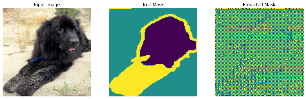
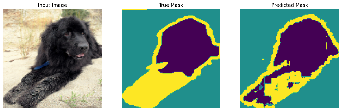
トレーニングする前に、モデルが何を予測するかを試してみましょう。
def create_mask(pred_mask):
  pred_mask = tf.math.argmax(pred_mask, axis=-1)
  pred_mask = pred_mask[..., tf.newaxis]
  return pred_mask[0]
def show_predictions(dataset=None, num=1):
  if dataset:
    for image, mask in dataset.take(num):
      pred_mask = model.predict(image)
      display([image[0], mask[0], create_mask(pred_mask)])
  else:
    display([sample_image, sample_mask,
             create_mask(model.predict(sample_image[tf.newaxis, ...]))])
show_predictions()
1/1 [==============================] - 3s 3s/step
以下に定義されるコールバックは、トレーニング中にモデルがどのように改善するかを観測するために使用されます。
class DisplayCallback(tf.keras.callbacks.Callback):
  def on_epoch_end(self, epoch, logs=None):
    clear_output(wait=True)
    show_predictions()
    print ('\nSample Prediction after epoch {}\n'.format(epoch+1))
EPOCHS = 20
VAL_SUBSPLITS = 5
VALIDATION_STEPS = info.splits['test'].num_examples//BATCH_SIZE//VAL_SUBSPLITS

model_history = model.fit(train_batches, epochs=EPOCHS,
                          steps_per_epoch=STEPS_PER_EPOCH,
                          validation_steps=VALIDATION_STEPS,
                          validation_data=test_batches,
                          callbacks=[DisplayCallback()])
1/1 [==============================] - 0s 47ms/step
Sample Prediction after epoch 20

57/57 [==============================] - 8s 140ms/step - loss: 0.1712 - accuracy: 0.9302 - val_loss: 0.2666 - val_accuracy: 0.9043
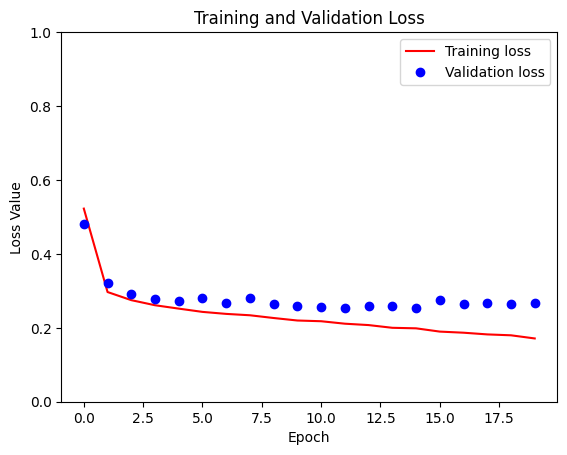
loss = model_history.history['loss']
val_loss = model_history.history['val_loss']

plt.figure()
plt.plot(model_history.epoch, loss, 'r', label='Training loss')
plt.plot(model_history.epoch, val_loss, 'bo', label='Validation loss')
plt.title('Training and Validation Loss')
plt.xlabel('Epoch')
plt.ylabel('Loss Value')
plt.ylim([0, 1])
plt.legend()
plt.show()
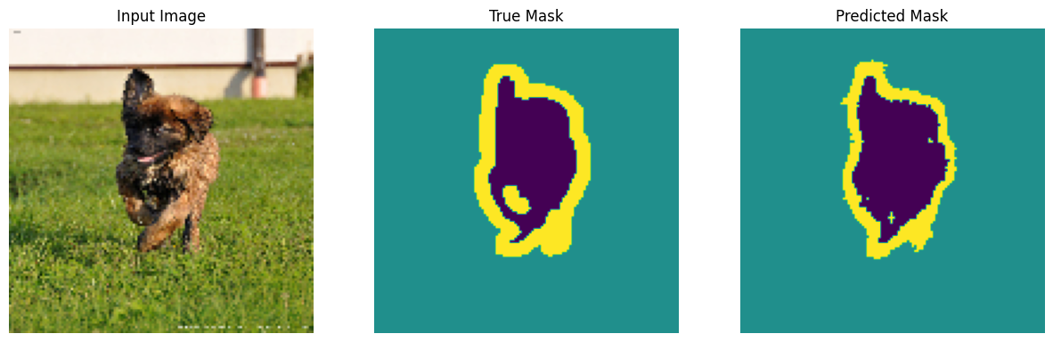
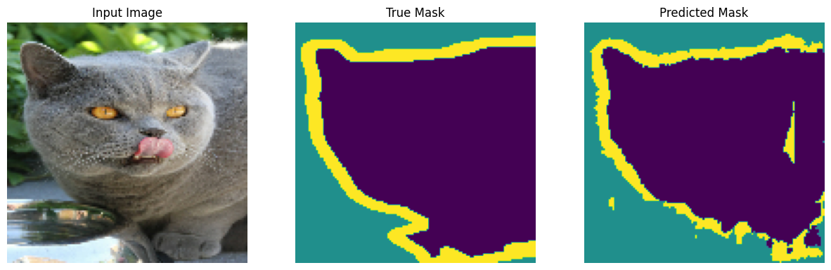
予測する
いくつか予測を行ってみましょう。時間の節約重視の場合はエポック数を少なくしますが、高精度の結果重視の場合はエポック数を増やして設定します。
show_predictions(test_batches, 3)
2/2 [==============================] - 0s 26ms/step
2/2 [==============================] - 0s 34ms/step
2/2 [==============================] - 0s 37ms/step
オプション: 不均衡なクラスとクラスの重み
セマンティックセグメンテーションデータセットは非常に不均衡であり、特定のクラスピクセルが他のクラスに比べて画像の内側寄りに存在する可能性があります。セグメンテーションの問題はピクセル単位の分類問題として対応することができるため、不均衡性を考慮して損失関数を重み付けすることで、不均衡の問題に対処することができます。単純かつエレガントにこの問題に取り組むことができます。詳細は、不均衡なデータでの分類のチュートリアルをご覧ください。
あいまいさを回避するために、Model.fit は 3 次元以上のターゲットの class_weight 引数をサポートしていません。
try:
  model_history = model.fit(train_batches, epochs=EPOCHS,
                            steps_per_epoch=STEPS_PER_EPOCH,
                            class_weight = {0:2.0, 1:2.0, 2:1.0})
  assert False
except Exception as e:
  print(f"Expected {type(e).__name__}: {e}")
Epoch 1/20
57/57 [==============================] - 8s 113ms/step - loss: 0.2599 - accuracy: 0.9219
Epoch 2/20
57/57 [==============================] - 6s 115ms/step - loss: 0.2628 - accuracy: 0.9209
Epoch 3/20
57/57 [==============================] - 7s 116ms/step - loss: 0.2417 - accuracy: 0.9260
Epoch 4/20
57/57 [==============================] - 7s 117ms/step - loss: 0.2394 - accuracy: 0.9265
Epoch 5/20
57/57 [==============================] - 7s 116ms/step - loss: 0.2242 - accuracy: 0.9304
Epoch 6/20
57/57 [==============================] - 7s 114ms/step - loss: 0.2196 - accuracy: 0.9316
Epoch 7/20
57/57 [==============================] - 6s 114ms/step - loss: 0.2126 - accuracy: 0.9334
Epoch 8/20
57/57 [==============================] - 6s 113ms/step - loss: 0.2037 - accuracy: 0.9358
Epoch 9/20
57/57 [==============================] - 6s 112ms/step - loss: 0.1960 - accuracy: 0.9377
Epoch 10/20
57/57 [==============================] - 6s 112ms/step - loss: 0.1914 - accuracy: 0.9391
Epoch 11/20
57/57 [==============================] - 6s 112ms/step - loss: 0.1921 - accuracy: 0.9390
Epoch 12/20
57/57 [==============================] - 6s 112ms/step - loss: 0.1860 - accuracy: 0.9406
Epoch 13/20
57/57 [==============================] - 6s 112ms/step - loss: 0.1780 - accuracy: 0.9430
Epoch 14/20
57/57 [==============================] - 6s 113ms/step - loss: 0.1734 - accuracy: 0.9442
Epoch 15/20
57/57 [==============================] - 6s 113ms/step - loss: 0.1722 - accuracy: 0.9448
Epoch 16/20
57/57 [==============================] - 6s 113ms/step - loss: 0.1685 - accuracy: 0.9457
Epoch 17/20
57/57 [==============================] - 6s 114ms/step - loss: 0.1624 - accuracy: 0.9477
Epoch 18/20
57/57 [==============================] - 6s 114ms/step - loss: 0.1589 - accuracy: 0.9487
Epoch 19/20
57/57 [==============================] - 6s 113ms/step - loss: 0.1576 - accuracy: 0.9492
Epoch 20/20
57/57 [==============================] - 6s 113ms/step - loss: 0.1510 - accuracy: 0.9512
Expected AssertionError:
そのため、この場合、自分で重み付けを実装する必要があります。これにはサンプルの重み付けを使用します。Model.fit は (data, label) ペアのほかに (data, label, sample_weight) トリプレットも受け入れます。
Keras Model.fit は sample_weight を損失とメトリクスに伝搬しますが、sample_weight 引数も受け入れます。サンプル重みは、縮小ステップの前にサンプル値で乗算されます。以下に例を示します。
label = [0,0]
prediction = [[-3., 0], [-3, 0]]
sample_weight = [1, 10]

loss = tf.keras.losses.SparseCategoricalCrossentropy(from_logits=True,
                                               reduction=tf.keras.losses.Reduction.NONE)
loss(label, prediction, sample_weight).numpy()
array([ 3.0485873, 30.485874 ], dtype=float32)
つまり、このチュートリアルのサンプル重みを作るには、(data, label) ペアを取って (data, label, sample_weight) トリプルを返す関数が必要となります。sample_weight は各ピクセルのクラス重みを含む 1-channel の画像です。
実装を可能な限り単純にするために、ラベルをclass_weight リストのインデックスとして使用します。
def add_sample_weights(image, label):
  # The weights for each class, with the constraint that:
  #     sum(class_weights) == 1.0
  class_weights = tf.constant([2.0, 2.0, 1.0])
  class_weights = class_weights/tf.reduce_sum(class_weights)

  # Create an image of `sample_weights` by using the label at each pixel as an
  # index into the `class weights` .
  sample_weights = tf.gather(class_weights, indices=tf.cast(label, tf.int32))

  return image, label, sample_weights
この結果、データセットの各要素には、3 つの画像が含まれます。
train_batches.map(add_sample_weights).element_spec
(TensorSpec(shape=(None, 128, 128, 3), dtype=tf.float32, name=None),
 TensorSpec(shape=(None, 128, 128, 1), dtype=tf.float32, name=None),
 TensorSpec(shape=(None, 128, 128, 1), dtype=tf.float32, name=None))
次に、この重み付けが付けられたデータセットでモデルをトレーニングしてみましょう。
weighted_model = unet_model(OUTPUT_CLASSES)
weighted_model.compile(
    optimizer='adam',
    loss=tf.keras.losses.SparseCategoricalCrossentropy(from_logits=True),
    metrics=['accuracy'])
weighted_model.fit(
    train_batches.map(add_sample_weights),
    epochs=1,
    steps_per_epoch=10)
10/10 [==============================] - 5s 118ms/step - loss: 0.2782 - accuracy: 0.6484
<keras.src.callbacks.History at 0x7f8ebaeba3a0>
次のステップ
これで画像セグメンテーションとは何か、それがどのように機能するかについての知識が得られたはずです。このチュートリアルは、異なる中間レイヤー出力や、異なる事前トレーニング済みモデルでも試すことができます。また、Kaggle がホストしている Carvana 画像マスキングチャレンジに挑戦してみることもお勧めです。
Tensorflow Object Detection API を参照して、独自のデータで再トレーニング可能な別のモデルを確認するのも良いでしょう。トレーニング済みのモデルは、TensorFlow Hub にあります。