
|
|
|
 View source on GitHub View source on GitHub
|
|
Overview
The tf.distribute.Strategy API provides an abstraction for distributing your training across multiple processing units. It allows you to carry out distributed training using existing models and training code with minimal changes.
This tutorial demonstrates how to use the tf.distribute.MirroredStrategy to perform in-graph replication with synchronous training on many GPUs on one machine. The strategy essentially copies all of the model's variables to each processor. Then, it uses all-reduce to combine the gradients from all processors, and applies the combined value to all copies of the model.
You will use the tf.keras APIs to build the model and Model.fit for training it. (To learn about distributed training with a custom training loop and the MirroredStrategy, check out this tutorial.)
MirroredStrategy trains your model on multiple GPUs on a single machine. For synchronous training on many GPUs on multiple workers, use the tf.distribute.MultiWorkerMirroredStrategy with the Keras Model.fit or a custom training loop. For other options, refer to the Distributed training guide.
To learn about various other strategies, there is the Distributed training with TensorFlow guide.
Setup
import tensorflow_datasets as tfds
import tensorflow as tf

import os

# Load the TensorBoard notebook extension.
%load_ext tensorboard
print(tf.__version__)
Download the dataset
Load the MNIST dataset from TensorFlow Datasets. This returns a dataset in the tf.data format.
Setting the with_info argument to True includes the metadata for the entire dataset, which is being saved here to info. Among other things, this metadata object includes the number of train and test examples.
datasets, info = tfds.load(name='mnist', with_info=True, as_supervised=True)

mnist_train, mnist_test = datasets['train'], datasets['test']
Define the distribution strategy
Create a MirroredStrategy object. This will handle distribution and provide a context manager (MirroredStrategy.scope) to build your model inside.
strategy = tf.distribute.MirroredStrategy()
print('Number of devices: {}'.format(strategy.num_replicas_in_sync))
Set up the input pipeline
When training a model with multiple GPUs, you can use the extra computing power effectively by increasing the batch size. In general, use the largest batch size that fits the GPU memory and tune the learning rate accordingly.
# You can also do info.splits.total_num_examples to get the total
# number of examples in the dataset.

num_train_examples = info.splits['train'].num_examples
num_test_examples = info.splits['test'].num_examples

BUFFER_SIZE = 10000

BATCH_SIZE_PER_REPLICA = 64
BATCH_SIZE = BATCH_SIZE_PER_REPLICA * strategy.num_replicas_in_sync
Define a function that normalizes the image pixel values from the [0, 255] range to the [0, 1] range (feature scaling):
def scale(image, label):
  image = tf.cast(image, tf.float32)
  image /= 255

  return image, label
Apply this scale function to the training and test data, and then use the tf.data.Dataset APIs to shuffle the training data (Dataset.shuffle), and batch it (Dataset.batch). Notice that you are also keeping an in-memory cache of the training data to improve performance (Dataset.cache).
train_dataset = mnist_train.map(scale).cache().shuffle(BUFFER_SIZE).batch(BATCH_SIZE)
eval_dataset = mnist_test.map(scale).batch(BATCH_SIZE)
Create the model and instantiate the optimizer
Within the context of Strategy.scope, create and compile the model using the Keras API:
with strategy.scope():
  model = tf.keras.Sequential([
      tf.keras.layers.Conv2D(32, 3, activation='relu', input_shape=(28, 28, 1)),
      tf.keras.layers.MaxPooling2D(),
      tf.keras.layers.Flatten(),
      tf.keras.layers.Dense(64, activation='relu'),
      tf.keras.layers.Dense(10)
  ])

  model.compile(loss=tf.keras.losses.SparseCategoricalCrossentropy(from_logits=True),
                optimizer=tf.keras.optimizers.Adam(learning_rate=0.001),
                metrics=['accuracy'])
For this toy example with the MNIST dataset, you will be using the Adam optimizer's default learning rate of 0.001.
For larger datasets, the key benefit of distributed training is to learn more in each training step, because each step processes more training data in parallel, which allows for a larger learning rate (within the limits of the model and dataset).
Define the callbacks
Define the following Keras Callbacks:
tf.keras.callbacks.TensorBoard: writes a log for TensorBoard, which allows you to visualize the graphs.tf.keras.callbacks.ModelCheckpoint: saves the model at a certain frequency, such as after every epoch.tf.keras.callbacks.BackupAndRestore: provides the fault tolerance functionality by backing up the model and current epoch number. Learn more in the Fault tolerance section of the Multi-worker training with Keras tutorial.tf.keras.callbacks.LearningRateScheduler: schedules the learning rate to change after, for example, every epoch/batch.
For illustrative purposes, add a custom callback called PrintLR to display the learning rate in the notebook.
# Define the checkpoint directory to store the checkpoints.
checkpoint_dir = './training_checkpoints'
# Define the name of the checkpoint files.
checkpoint_prefix = os.path.join(checkpoint_dir, "ckpt_{epoch}")
# Define a function for decaying the learning rate.
# You can define any decay function you need.
def decay(epoch):
  if epoch < 3:
    return 1e-3
  elif epoch >= 3 and epoch < 7:
    return 1e-4
  else:
    return 1e-5
# Define a callback for printing the learning rate at the end of each epoch.
class PrintLR(tf.keras.callbacks.Callback):
  def on_epoch_end(self, epoch, logs=None):
    print('\nLearning rate for epoch {} is {}'.format(        epoch + 1, model.optimizer.lr.numpy()))
# Put all the callbacks together.
callbacks = [
    tf.keras.callbacks.TensorBoard(log_dir='./logs'),
    tf.keras.callbacks.ModelCheckpoint(filepath=checkpoint_prefix,
                                       save_weights_only=True),
    tf.keras.callbacks.LearningRateScheduler(decay),
    PrintLR()
]
Train and evaluate
Now, train the model in the usual way by calling Keras Model.fit on the model and passing in the dataset created at the beginning of the tutorial. This step is the same whether you are distributing the training or not.
EPOCHS = 12

model.fit(train_dataset, epochs=EPOCHS, callbacks=callbacks)
Check for saved checkpoints:
# Check the checkpoint directory.ls {checkpoint_dir}
To check how well the model performs, load the latest checkpoint and call Model.evaluate on the test data:
model.load_weights(tf.train.latest_checkpoint(checkpoint_dir))

eval_loss, eval_acc = model.evaluate(eval_dataset)

print('Eval loss: {}, Eval accuracy: {}'.format(eval_loss, eval_acc))
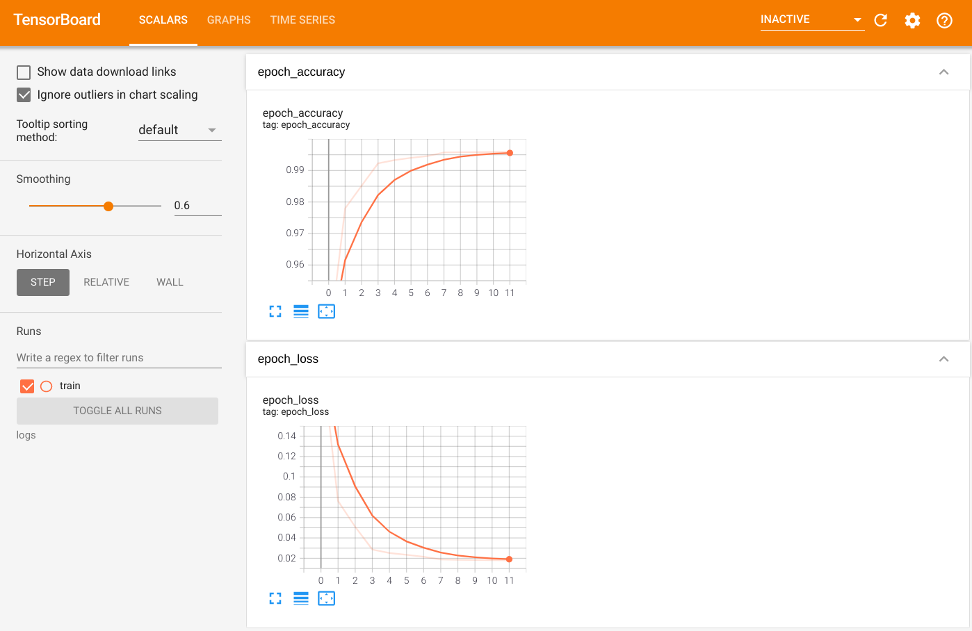
To visualize the output, launch TensorBoard and view the logs:
%tensorboard --logdir=logs
ls -sh ./logsSave the model
Save the model to a .keras zip archive using Model.save. After your model is saved, you can load it with or without the Strategy.scope.
path = 'my_model.keras'
model.save(path)
Now, load the model without Strategy.scope:
unreplicated_model = tf.keras.models.load_model(path)

unreplicated_model.compile(
    loss=tf.keras.losses.SparseCategoricalCrossentropy(from_logits=True),
    optimizer=tf.keras.optimizers.Adam(),
    metrics=['accuracy'])

eval_loss, eval_acc = unreplicated_model.evaluate(eval_dataset)

print('Eval loss: {}, Eval Accuracy: {}'.format(eval_loss, eval_acc))
Load the model with Strategy.scope:
with strategy.scope():
  replicated_model = tf.keras.models.load_model(path)
  replicated_model.compile(loss=tf.keras.losses.SparseCategoricalCrossentropy(from_logits=True),
                           optimizer=tf.keras.optimizers.Adam(),
                           metrics=['accuracy'])

  eval_loss, eval_acc = replicated_model.evaluate(eval_dataset)
  print ('Eval loss: {}, Eval Accuracy: {}'.format(eval_loss, eval_acc))
Additional resources
More examples that use different distribution strategies with the Keras Model.fit API:
- The Solve GLUE tasks using BERT on TPU tutorial uses
tf.distribute.MirroredStrategyfor training on GPUs andtf.distribute.TPUStrategyon TPUs. - The Save and load a model using a distribution strategy tutorial demonstates how to use the SavedModel APIs with
tf.distribute.Strategy. - The official TensorFlow models can be configured to run multiple distribution strategies.
To learn more about TensorFlow distribution strategies:
- The Custom training with tf.distribute.Strategy tutorial shows how to use the
tf.distribute.MirroredStrategyfor single-worker training with a custom training loop. - The Multi-worker training with Keras tutorial shows how to use the
MultiWorkerMirroredStrategywithModel.fit. - The Custom training loop with Keras and MultiWorkerMirroredStrategy tutorial shows how to use the
MultiWorkerMirroredStrategywith Keras and a custom training loop. - The Distributed training in TensorFlow guide provides an overview of the available distribution strategies.
- The Better performance with tf.function guide provides information about other strategies and tools, such as the TensorFlow Profiler you can use to optimize the performance of your TensorFlow models.