Adversarial example using FGSM

This tutorial creates an adversarial example using the Fast Gradient Signed Method (FGSM) attack as described in Explaining and Harnessing Adversarial Examples by Goodfellow et al. This was one of the first and most popular attacks to fool a neural network.

What is an adversarial example?

Adversarial examples are specialised inputs created with the purpose of confusing a neural network, resulting in the misclassification of a given input. These notorious inputs are indistinguishable to the human eye, but cause the network to fail to identify the contents of the image. There are several types of such attacks, however, here the focus is on the fast gradient sign method attack, which is a white box attack whose goal is to ensure misclassification. A white box attack is where the attacker has complete access to the model being attacked. One of the most famous examples of an adversarial image shown below is taken from the aforementioned paper.

Adversarial Example

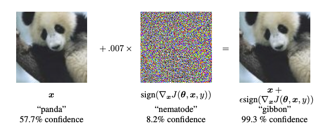
Here, starting with the image of a panda, the attacker adds small perturbations (distortions) to the original image, which results in the model labelling this image as a gibbon, with high confidence. The process of adding these perturbations is explained below.

Fast gradient sign method

The fast gradient sign method works by using the gradients of the neural network to create an adversarial example. For an input image, the method uses the gradients of the loss with respect to the input image to create a new image that maximises the loss. This new image is called the adversarial image. This can be summarised using the following expression:

\[adv\_x = x + \epsilon*\text{sign}(\nabla_xJ(\theta, x, y))\]

where

adv_x : Adversarial image.
x : Original input image.
y : Original input label.
\(\epsilon\) : Multiplier to ensure the perturbations are small.
\(\theta\) : Model parameters.
\(J\) : Loss.

An intriguing property here, is the fact that the gradients are taken with respect to the input image. This is done because the objective is to create an image that maximises the loss. A method to accomplish this is to find how much each pixel in the image contributes to the loss value, and add a perturbation accordingly. This works pretty fast because it is easy to find how each input pixel contributes to the loss by using the chain rule and finding the required gradients. Hence, the gradients are taken with respect to the image. In addition, since the model is no longer being trained (thus the gradient is not taken with respect to the trainable variables, i.e., the model parameters), and so the model parameters remain constant. The only goal is to fool an already trained model.

So let's try and fool a pretrained model. In this tutorial, the model is MobileNetV2 model, pretrained on ImageNet.

import tensorflow as tf
import matplotlib as mpl
import matplotlib.pyplot as plt

mpl.rcParams['figure.figsize'] = (8, 8)
mpl.rcParams['axes.grid'] = False

2025-12-01 04:41:58.040684: E external/local_xla/xla/stream_executor/cuda/cuda_fft.cc:467] Unable to register cuFFT factory: Attempting to register factory for plugin cuFFT when one has already been registered
WARNING: All log messages before absl::InitializeLog() is called are written to STDERR
E0000 00:00:1764564118.063167  298228 cuda_dnn.cc:8579] Unable to register cuDNN factory: Attempting to register factory for plugin cuDNN when one has already been registered
E0000 00:00:1764564118.070434  298228 cuda_blas.cc:1407] Unable to register cuBLAS factory: Attempting to register factory for plugin cuBLAS when one has already been registered
W0000 00:00:1764564118.088432  298228 computation_placer.cc:177] computation placer already registered. Please check linkage and avoid linking the same target more than once.
W0000 00:00:1764564118.088452  298228 computation_placer.cc:177] computation placer already registered. Please check linkage and avoid linking the same target more than once.
W0000 00:00:1764564118.088455  298228 computation_placer.cc:177] computation placer already registered. Please check linkage and avoid linking the same target more than once.
W0000 00:00:1764564118.088457  298228 computation_placer.cc:177] computation placer already registered. Please check linkage and avoid linking the same target more than once.

Let's load the pretrained MobileNetV2 model and the ImageNet class names.

pretrained_model = tf.keras.applications.MobileNetV2(include_top=True,
                                                     weights='imagenet')
pretrained_model.trainable = False

# ImageNet labels
decode_predictions = tf.keras.applications.mobilenet_v2.decode_predictions

I0000 00:00:1764564122.575880  298228 gpu_device.cc:2019] Created device /job:localhost/replica:0/task:0/device:GPU:0 with 13638 MB memory:  -> device: 0, name: Tesla T4, pci bus id: 0000:00:05.0, compute capability: 7.5
I0000 00:00:1764564122.578188  298228 gpu_device.cc:2019] Created device /job:localhost/replica:0/task:0/device:GPU:1 with 13756 MB memory:  -> device: 1, name: Tesla T4, pci bus id: 0000:00:06.0, compute capability: 7.5
I0000 00:00:1764564122.580612  298228 gpu_device.cc:2019] Created device /job:localhost/replica:0/task:0/device:GPU:2 with 13756 MB memory:  -> device: 2, name: Tesla T4, pci bus id: 0000:00:07.0, compute capability: 7.5
I0000 00:00:1764564122.582819  298228 gpu_device.cc:2019] Created device /job:localhost/replica:0/task:0/device:GPU:3 with 13756 MB memory:  -> device: 3, name: Tesla T4, pci bus id: 0000:00:08.0, compute capability: 7.5
Downloading data from https://storage.googleapis.com/tensorflow/keras-applications/mobilenet_v2/mobilenet_v2_weights_tf_dim_ordering_tf_kernels_1.0_224.h5
14536120/14536120 ━━━━━━━━━━━━━━━━━━━━ 0s 0us/step

# Helper function to preprocess the image so that it can be inputted in MobileNetV2
def preprocess(image):
  image = tf.cast(image, tf.float32)
  image = tf.image.resize(image, (224, 224))
  image = tf.keras.applications.mobilenet_v2.preprocess_input(image)
  image = image[None, ...]
  return image

# Helper function to extract labels from probability vector
def get_imagenet_label(probs):
  return decode_predictions(probs, top=1)[0][0]

Original image

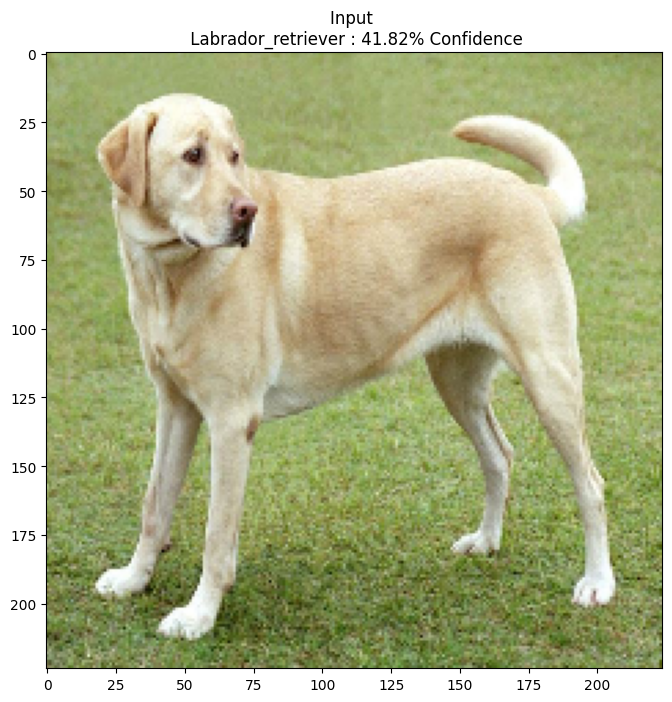
Let's use a sample image of a Labrador Retriever by Mirko CC-BY-SA 3.0 from Wikimedia Common and create adversarial examples from it. The first step is to preprocess it so that it can be fed as an input to the MobileNetV2 model.

image_path = tf.keras.utils.get_file('YellowLabradorLooking_new.jpg', 'https://storage.googleapis.com/download.tensorflow.org/example_images/YellowLabradorLooking_new.jpg')
image_raw = tf.io.read_file(image_path)
image = tf.image.decode_image(image_raw)

image = preprocess(image)
image_probs = pretrained_model.predict(image)

WARNING: All log messages before absl::InitializeLog() is called are written to STDERR
I0000 00:00:1764564126.041831  298392 service.cc:152] XLA service 0x7f67800025b0 initialized for platform CUDA (this does not guarantee that XLA will be used). Devices:
I0000 00:00:1764564126.041864  298392 service.cc:160]   StreamExecutor device (0): Tesla T4, Compute Capability 7.5
I0000 00:00:1764564126.041868  298392 service.cc:160]   StreamExecutor device (1): Tesla T4, Compute Capability 7.5
I0000 00:00:1764564126.041870  298392 service.cc:160]   StreamExecutor device (2): Tesla T4, Compute Capability 7.5
I0000 00:00:1764564126.041873  298392 service.cc:160]   StreamExecutor device (3): Tesla T4, Compute Capability 7.5
I0000 00:00:1764564126.582594  298392 cuda_dnn.cc:529] Loaded cuDNN version 91600
2025-12-01 04:42:11.939825: E external/local_xla/xla/stream_executor/cuda/cuda_timer.cc:86] Delay kernel timed out: measured time has sub-optimal accuracy. There may be a missing warmup execution, please investigate in Nsight Systems.
2025-12-01 04:42:12.073314: E external/local_xla/xla/stream_executor/cuda/cuda_timer.cc:86] Delay kernel timed out: measured time has sub-optimal accuracy. There may be a missing warmup execution, please investigate in Nsight Systems.
I0000 00:00:1764564133.397688  298392 device_compiler.h:188] Compiled cluster using XLA!  This line is logged at most once for the lifetime of the process.
1/1 ━━━━━━━━━━━━━━━━━━━━ 9s 9s/step

Let's have a look at the image.

plt.figure()
plt.imshow(image[0] * 0.5 + 0.5)  # To change [-1, 1] to [0,1]
_, image_class, class_confidence = get_imagenet_label(image_probs)
plt.title('{} : {:.2f}% Confidence'.format(image_class, class_confidence*100))
plt.show()

png

Create the adversarial image

Implementing fast gradient sign method

The first step is to create perturbations which will be used to distort the original image resulting in an adversarial image. As mentioned, for this task, the gradients are taken with respect to the image.

loss_object = tf.keras.losses.CategoricalCrossentropy()

def create_adversarial_pattern(input_image, input_label):
  with tf.GradientTape() as tape:
    tape.watch(input_image)
    prediction = pretrained_model(input_image)
    loss = loss_object(input_label, prediction)

  # Get the gradients of the loss w.r.t to the input image.
  gradient = tape.gradient(loss, input_image)
  # Get the sign of the gradients to create the perturbation
  signed_grad = tf.sign(gradient)
  return signed_grad

The resulting perturbations can also be visualised.

# Get the input label of the image.
labrador_retriever_index = 208
label = tf.one_hot(labrador_retriever_index, image_probs.shape[-1])
label = tf.reshape(label, (1, image_probs.shape[-1]))

perturbations = create_adversarial_pattern(image, label)
plt.imshow(perturbations[0] * 0.5 + 0.5);  # To change [-1, 1] to [0,1]

png

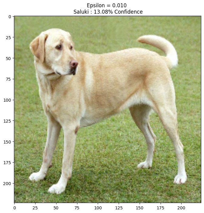
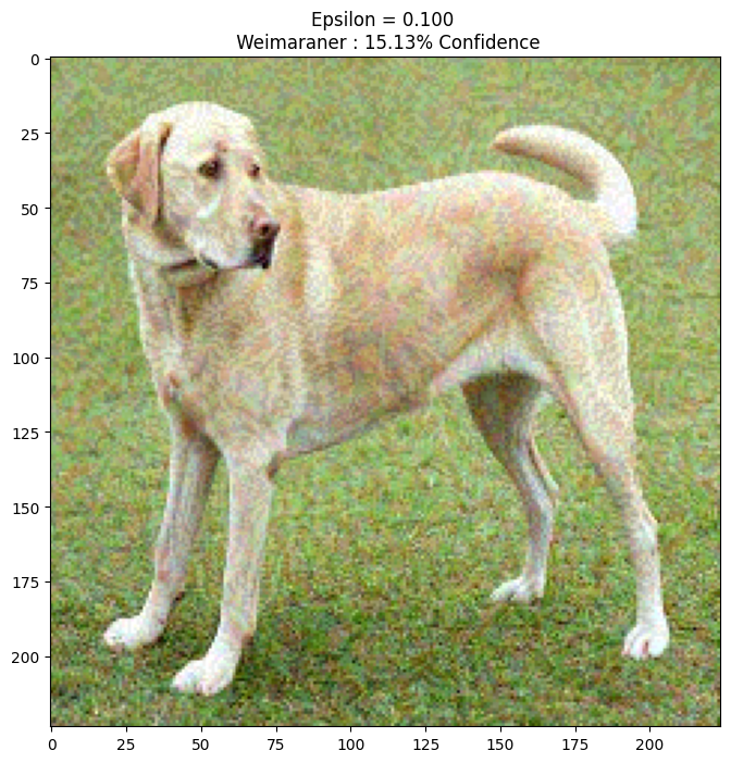
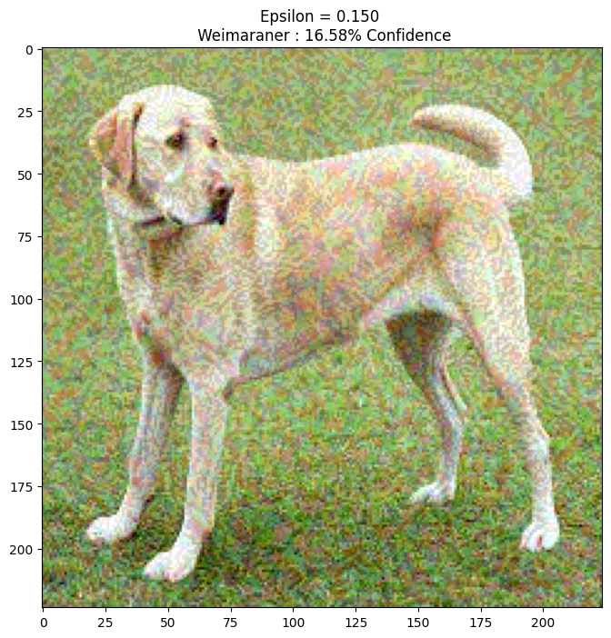
Let's try this out for different values of epsilon and observe the resultant image. You'll notice that as the value of epsilon is increased, it becomes easier to fool the network. However, this comes as a trade-off which results in the perturbations becoming more identifiable.

def display_images(image, description):
  _, label, confidence = get_imagenet_label(pretrained_model.predict(image))
  plt.figure()
  plt.imshow(image[0]*0.5+0.5)
  plt.title('{} \n {} : {:.2f}% Confidence'.format(description,
                                                   label, confidence*100))
  plt.show()

epsilons = [0, 0.01, 0.1, 0.15]
descriptions = [('Epsilon = {:0.3f}'.format(eps) if eps else 'Input')
                for eps in epsilons]

for i, eps in enumerate(epsilons):
  adv_x = image + eps*perturbations
  adv_x = tf.clip_by_value(adv_x, -1, 1)
  display_images(adv_x, descriptions[i])

1/1 ━━━━━━━━━━━━━━━━━━━━ 0s 81ms/step

png

1/1 ━━━━━━━━━━━━━━━━━━━━ 0s 78ms/step

png

1/1 ━━━━━━━━━━━━━━━━━━━━ 0s 78ms/step

png

1/1 ━━━━━━━━━━━━━━━━━━━━ 0s 78ms/step

png

Next steps

Now that you know about adversarial attacks, try this out on different datasets and different architectures. You may also create and train your own model, and then attempt to fool it using the same method. You can also try and see how the confidence in predictions vary as you change epsilon.

Though powerful, the attack shown in this tutorial was just the start of research into adversarial attacks, and there have been multiple papers creating more powerful attacks since then. In addition to adversarial attacks, research has also led to the creation of defenses, which aims at creating robust machine learning models. You may review this survey paper for a comprehensive list of adversarial attacks and defences.

For many more implementations of adversarial attacks and defenses, you may want to see the adversarial example library CleverHans.

Adversarial example using FGSM Stay organized with collections Save and categorize content based on your preferences.