تور احتمالات TensorFlow

مشاهده در TensorFlow.org

در Google Colab اجرا شود

مشاهده منبع در GitHub

دانلود دفترچه یادداشت

در این Colab، ما برخی از ویژگی های اساسی TensorFlow Probability را بررسی می کنیم.

وابستگی ها و پیش نیازها

وارد كردن

from pprint import pprint
import matplotlib.pyplot as plt
import numpy as np
import seaborn as sns

import tensorflow.compat.v2 as tf
tf.enable_v2_behavior()

import tensorflow_probability as tfp

sns.reset_defaults()
sns.set_context(context='talk',font_scale=0.7)
plt.rcParams['image.cmap'] = 'viridis'

%matplotlib inline

tfd = tfp.distributions
tfb = tfp.bijectors

Utils

def print_subclasses_from_module(module, base_class, maxwidth=80):
  import functools, inspect, sys
  subclasses = [name for name, obj in inspect.getmembers(module)
                if inspect.isclass(obj) and issubclass(obj, base_class)]
  def red(acc, x):
    if not acc or len(acc[-1]) + len(x) + 2 > maxwidth:
      acc.append(x)
    else:
      acc[-1] += ", " + x
    return acc
  print('\n'.join(functools.reduce(red, subclasses, [])))

طرح کلی

• تنسورفلو
• احتمال TensorFlow
  • توزیع ها
  • بیژکتورها
  • MCMC
  • ...و بیشتر!

مقدمه: تنسورفلو

TensorFlow یک کتابخانه محاسباتی علمی است.

پشتیبانی می کند

• تعداد زیادی عملیات ریاضی
• محاسبات برداری کارآمد
• شتاب سخت افزاری آسان
• تمایز خودکار

برداری

• وکتوری شدن همه چیز را سریع می کند!
• همچنین به این معنی است که ما در مورد اشکال زیاد فکر می کنیم

mats = tf.random.uniform(shape=[1000, 10, 10])
vecs = tf.random.uniform(shape=[1000, 10, 1])

def for_loop_solve():
  return np.array(
    [tf.linalg.solve(mats[i, ...], vecs[i, ...]) for i in range(1000)])

def vectorized_solve():
  return tf.linalg.solve(mats, vecs)

# Vectorization for the win!
%timeit for_loop_solve()
%timeit vectorized_solve()

1 loops, best of 3: 2 s per loop
1000 loops, best of 3: 653 µs per loop

شتاب سخت افزاری

# Code can run seamlessly on a GPU, just change Colab runtime type
# in the 'Runtime' menu.
if tf.test.gpu_device_name() == '/device:GPU:0':
  print("Using a GPU")
else:
  print("Using a CPU")

Using a CPU

تمایز خودکار

a = tf.constant(np.pi)
b = tf.constant(np.e)
with tf.GradientTape() as tape:
  tape.watch([a, b])
  c = .5 * (a**2 + b**2)
grads = tape.gradient(c, [a, b])
print(grads[0])
print(grads[1])

tf.Tensor(3.1415927, shape=(), dtype=float32)
tf.Tensor(2.7182817, shape=(), dtype=float32)

احتمال TensorFlow

TensorFlow Probability کتابخانه ای برای استدلال احتمالی و تجزیه و تحلیل آماری در TensorFlow است.

ما مدل سازی، استنباط، و نقد از طریق ترکیب قطعات مدولار سطح پایین را پشتیبانی کند.

بلوک های ساختمانی سطح پایین

• توزیع ها
• بیژکتورها

ساختارهای سطح بالا (er)

• زنجیره مارکوف مونت کارلو
• لایه های احتمالی
• سری زمانی ساختاری
• مدل های خطی تعمیم یافته
• بهینه سازها

توزیع ها

tfp.distributions.Distribution : یک کلاس با دو روش اصلی این است که sample و log_prob .

TFP توزیع های زیادی دارد!

print_subclasses_from_module(tfp.distributions, tfp.distributions.Distribution)

Autoregressive, BatchReshape, Bates, Bernoulli, Beta, BetaBinomial, Binomial
Blockwise, Categorical, Cauchy, Chi, Chi2, CholeskyLKJ, ContinuousBernoulli
Deterministic, Dirichlet, DirichletMultinomial, Distribution, DoublesidedMaxwell
Empirical, ExpGamma, ExpRelaxedOneHotCategorical, Exponential, FiniteDiscrete
Gamma, GammaGamma, GaussianProcess, GaussianProcessRegressionModel
GeneralizedNormal, GeneralizedPareto, Geometric, Gumbel, HalfCauchy, HalfNormal
HalfStudentT, HiddenMarkovModel, Horseshoe, Independent, InverseGamma
InverseGaussian, JohnsonSU, JointDistribution, JointDistributionCoroutine
JointDistributionCoroutineAutoBatched, JointDistributionNamed
JointDistributionNamedAutoBatched, JointDistributionSequential
JointDistributionSequentialAutoBatched, Kumaraswamy, LKJ, Laplace
LinearGaussianStateSpaceModel, LogLogistic, LogNormal, Logistic, LogitNormal
Mixture, MixtureSameFamily, Moyal, Multinomial, MultivariateNormalDiag
MultivariateNormalDiagPlusLowRank, MultivariateNormalFullCovariance
MultivariateNormalLinearOperator, MultivariateNormalTriL
MultivariateStudentTLinearOperator, NegativeBinomial, Normal, OneHotCategorical
OrderedLogistic, PERT, Pareto, PixelCNN, PlackettLuce, Poisson
PoissonLogNormalQuadratureCompound, PowerSpherical, ProbitBernoulli
QuantizedDistribution, RelaxedBernoulli, RelaxedOneHotCategorical, Sample
SinhArcsinh, SphericalUniform, StudentT, StudentTProcess
TransformedDistribution, Triangular, TruncatedCauchy, TruncatedNormal, Uniform
VariationalGaussianProcess, VectorDeterministic, VonMises
VonMisesFisher, Weibull, WishartLinearOperator, WishartTriL, Zipf

یک اسکالر متغیره ساده Distribution

# A standard normal
normal = tfd.Normal(loc=0., scale=1.)
print(normal)

tfp.distributions.Normal("Normal", batch_shape=[], event_shape=[], dtype=float32)

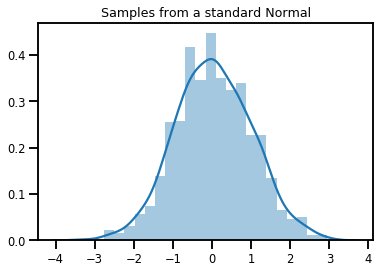
# Plot 1000 samples from a standard normal
samples = normal.sample(1000)
sns.distplot(samples)
plt.title("Samples from a standard Normal")
plt.show()

# Compute the log_prob of a point in the event space of `normal`
normal.log_prob(0.)

<tf.Tensor: shape=(), dtype=float32, numpy=-0.9189385>

# Compute the log_prob of a few points
normal.log_prob([-1., 0., 1.])

<tf.Tensor: shape=(3,), dtype=float32, numpy=array([-1.4189385, -0.9189385, -1.4189385], dtype=float32)>

توزیع ها و شکل ها

نامپای ndarrays و TensorFlow Tensors اشکال.

TensorFlow احتمال Distributions دارند معناشناسی شکل - شکل ما را به قطعات پارتیشن معنایی متمایز، حتی اگر همان تکه از حافظه ( Tensor / ndarray ) برای کل همه چیز استفاده می شود.

• شکل دسته ای نشان دهنده مجموعه ای از Distribution کنندگان با پارامترهای مشخص
• شکل رویداد نشان دهنده شکل نمونه از Distribution .

ما همیشه شکل‌های دسته‌ای را در سمت چپ و شکل‌های رویداد را در سمت راست قرار می‌دهیم.

دسته ای از اسکالر متغیره Distributions

دسته ها مانند توزیع های "بردار" هستند: نمونه های مستقلی که محاسبات آنها به صورت موازی اتفاق می افتد.

# Create a batch of 3 normals, and plot 1000 samples from each
normals = tfd.Normal([-2.5, 0., 2.5], 1.)  # The scale parameter broadacasts!
print("Batch shape:", normals.batch_shape)
print("Event shape:", normals.event_shape)

Batch shape: (3,)
Event shape: ()

# Samples' shapes go on the left!
samples = normals.sample(1000)
print("Shape of samples:", samples.shape)

Shape of samples: (1000, 3)

# Sample shapes can themselves be more complicated
print("Shape of samples:", normals.sample([10, 10, 10]).shape)

Shape of samples: (10, 10, 10, 3)

# A batch of normals gives a batch of log_probs.
print(normals.log_prob([-2.5, 0., 2.5]))

tf.Tensor([-0.9189385 -0.9189385 -0.9189385], shape=(3,), dtype=float32)

# The computation broadcasts, so a batch of normals applied to a scalar
# also gives a batch of log_probs.
print(normals.log_prob(0.))

tf.Tensor([-4.0439386 -0.9189385 -4.0439386], shape=(3,), dtype=float32)

# Normal numpy-like broadcasting rules apply!
xs = np.linspace(-6, 6, 200)
try:
  normals.log_prob(xs)
except Exception as e:
  print("TFP error:", e.message)

TFP error: Incompatible shapes: [200] vs. [3] [Op:SquaredDifference]

# That fails for the same reason this does:
try:
  np.zeros(200) + np.zeros(3)
except Exception as e:
  print("Numpy error:", e)

Numpy error: operands could not be broadcast together with shapes (200,) (3,)

# But this would work:
a = np.zeros([200, 1]) + np.zeros(3)
print("Broadcast shape:", a.shape)

Broadcast shape: (200, 3)

# And so will this!
xs = np.linspace(-6, 6, 200)[..., np.newaxis]
# => shape = [200, 1]

lps = normals.log_prob(xs)
print("Broadcast log_prob shape:", lps.shape)

Broadcast log_prob shape: (200, 3)

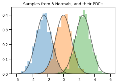
# Summarizing visually
for i in range(3):
  sns.distplot(samples[:, i], kde=False, norm_hist=True)
plt.plot(np.tile(xs, 3), normals.prob(xs), c='k', alpha=.5)
plt.title("Samples from 3 Normals, and their PDF's")
plt.show()

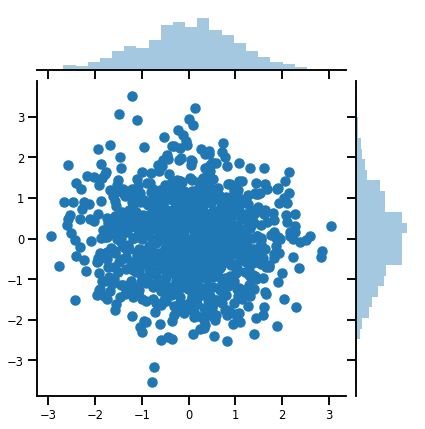
بردار متغیره Distribution

mvn = tfd.MultivariateNormalDiag(loc=[0., 0.], scale_diag = [1., 1.])
print("Batch shape:", mvn.batch_shape)
print("Event shape:", mvn.event_shape)

Batch shape: ()
Event shape: (2,)

samples = mvn.sample(1000)
print("Samples shape:", samples.shape)

Samples shape: (1000, 2)

g = sns.jointplot(samples[:, 0], samples[:, 1], kind='scatter')
plt.show()

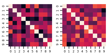
یک ماتریس متغیره Distribution

lkj = tfd.LKJ(dimension=10, concentration=[1.5, 3.0])
print("Batch shape: ", lkj.batch_shape)
print("Event shape: ", lkj.event_shape)

Batch shape:  (2,)
Event shape:  (10, 10)

samples = lkj.sample()
print("Samples shape: ", samples.shape)

Samples shape:  (2, 10, 10)

fig, axes = plt.subplots(nrows=1, ncols=2, figsize=(6, 3))
sns.heatmap(samples[0, ...], ax=axes[0], cbar=False)
sns.heatmap(samples[1, ...], ax=axes[1], cbar=False)
fig.tight_layout()
plt.show()

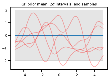
فرآیندهای گاوسی

kernel = tfp.math.psd_kernels.ExponentiatedQuadratic()
xs = np.linspace(-5., 5., 200).reshape([-1, 1])
gp = tfd.GaussianProcess(kernel, index_points=xs)
print("Batch shape:", gp.batch_shape)
print("Event shape:", gp.event_shape)

Batch shape: ()
Event shape: (200,)

upper, lower = gp.mean() + [2 * gp.stddev(), -2 * gp.stddev()]
plt.plot(xs, gp.mean())
plt.fill_between(xs[..., 0], upper, lower, color='k', alpha=.1)
for _ in range(5):
  plt.plot(xs, gp.sample(), c='r', alpha=.3)
plt.title(r"GP prior mean, $2\sigma$ intervals, and samples")
plt.show()

#    *** Bonus question ***
# Why do so many of these functions lie outside the 95% intervals?

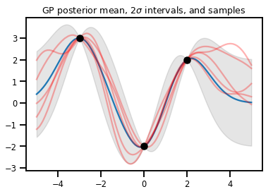
رگرسیون GP

# Suppose we have some observed data
obs_x = [[-3.], [0.], [2.]]  # Shape 3x1 (3 1-D vectors)
obs_y = [3., -2., 2.]        # Shape 3   (3 scalars)

gprm = tfd.GaussianProcessRegressionModel(kernel, xs, obs_x, obs_y)

upper, lower = gprm.mean() + [2 * gprm.stddev(), -2 * gprm.stddev()]
plt.plot(xs, gprm.mean())
plt.fill_between(xs[..., 0], upper, lower, color='k', alpha=.1)
for _ in range(5):
  plt.plot(xs, gprm.sample(), c='r', alpha=.3)
plt.scatter(obs_x, obs_y, c='k', zorder=3)
plt.title(r"GP posterior mean, $2\sigma$ intervals, and samples")
plt.show()

بیژکتورها

بیژکتورها (عمدتاً) عملکردهای معکوس و صاف را نشان می دهند. آنها را می توان برای تبدیل توزیع ها، حفظ توانایی نمونه برداری و محاسبه log_probs استفاده کرد. آنها می توانند در شود tfp.bijectors ماژول.

هر بیژکتور حداقل 3 روش را اجرا می کند:

• forward ،
• inverse ، و
• (حداقل) یکی از forward_log_det_jacobian و inverse_log_det_jacobian .

با این مواد، ما می‌توانیم توزیعی را تغییر دهیم و همچنان نمونه‌ها و پروب‌ها را از نتیجه دریافت کنیم!

در ریاضیات، تا حدودی شلخته

• \(X\) یک متغیر تصادفی با پی دی اف است \(p(x)\)
• \(g\) صاف، تابع وارون در فضای است \(X\)را
• \(Y = g(X)\) یک متغیر تصادفی تبدیل جدید است
• \(p(Y=y) = p(X=g^{-1}(y)) \cdot |\nabla g^{-1}(y)|\)

ذخیره سازی

Bijectors همچنین محاسبات رو به جلو و معکوس و log-det-Jacobians را در حافظه پنهان نگه می‌دارند که به ما امکان می‌دهد عملیات‌های بالقوه بسیار گران‌قیمت را تکرار کنیم!

print_subclasses_from_module(tfp.bijectors, tfp.bijectors.Bijector)

AbsoluteValue, Affine, AffineLinearOperator, AffineScalar, BatchNormalization
Bijector, Blockwise, Chain, CholeskyOuterProduct, CholeskyToInvCholesky
CorrelationCholesky, Cumsum, DiscreteCosineTransform, Exp, Expm1, FFJORD
FillScaleTriL, FillTriangular, FrechetCDF, GeneralizedExtremeValueCDF
GeneralizedPareto, GompertzCDF, GumbelCDF, Identity, Inline, Invert
IteratedSigmoidCentered, KumaraswamyCDF, LambertWTail, Log, Log1p
MaskedAutoregressiveFlow, MatrixInverseTriL, MatvecLU, MoyalCDF, NormalCDF
Ordered, Pad, Permute, PowerTransform, RationalQuadraticSpline, RayleighCDF
RealNVP, Reciprocal, Reshape, Scale, ScaleMatvecDiag, ScaleMatvecLU
ScaleMatvecLinearOperator, ScaleMatvecTriL, ScaleTriL, Shift, ShiftedGompertzCDF
Sigmoid, Sinh, SinhArcsinh, SoftClip, Softfloor, SoftmaxCentered, Softplus
Softsign, Split, Square, Tanh, TransformDiagonal, Transpose, WeibullCDF

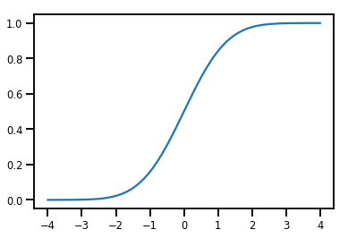
ساده Bijector

normal_cdf = tfp.bijectors.NormalCDF()
xs = np.linspace(-4., 4., 200)
plt.plot(xs, normal_cdf.forward(xs))
plt.show()

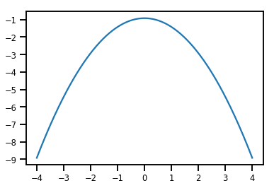
plt.plot(xs, normal_cdf.forward_log_det_jacobian(xs, event_ndims=0))
plt.show()

Bijector تبدیل یک Distribution

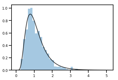
exp_bijector = tfp.bijectors.Exp()
log_normal = exp_bijector(tfd.Normal(0., .5))

samples = log_normal.sample(1000)
xs = np.linspace(1e-10, np.max(samples), 200)
sns.distplot(samples, norm_hist=True, kde=False)
plt.plot(xs, log_normal.prob(xs), c='k', alpha=.75)
plt.show()

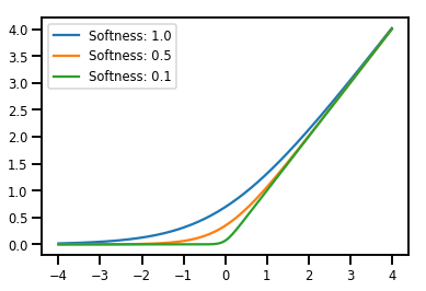
دوز مصالح Bijectors

# Create a batch of bijectors of shape [3,]
softplus = tfp.bijectors.Softplus(
  hinge_softness=[1., .5, .1])
print("Hinge softness shape:", softplus.hinge_softness.shape)

Hinge softness shape: (3,)

# For broadcasting, we want this to be shape [200, 1]
xs = np.linspace(-4., 4., 200)[..., np.newaxis]
ys = softplus.forward(xs)
print("Forward shape:", ys.shape)

Forward shape: (200, 3)

# Visualization
lines = plt.plot(np.tile(xs, 3), ys)
for line, hs in zip(lines, softplus.hinge_softness):
  line.set_label("Softness: %1.1f" % hs)
plt.legend()
plt.show()

ذخیره سازی

# This bijector represents a matrix outer product on the forward pass,
# and a cholesky decomposition on the inverse pass. The latter costs O(N^3)!
bij = tfb.CholeskyOuterProduct()

size = 2500
# Make a big, lower-triangular matrix
big_lower_triangular = tf.eye(size)
# Squaring it gives us a positive-definite matrix
big_positive_definite = bij.forward(big_lower_triangular)

# Caching for the win!
%timeit bij.inverse(big_positive_definite)
%timeit tf.linalg.cholesky(big_positive_definite)

10000 loops, best of 3: 114 µs per loop
1 loops, best of 3: 208 ms per loop

MCMC

TFP برای پشتیبانی از برخی از الگوریتم‌های استاندارد مونت کارلو زنجیره مارکوف، از جمله مونت کارلو همیلتونی ساخته شده است.

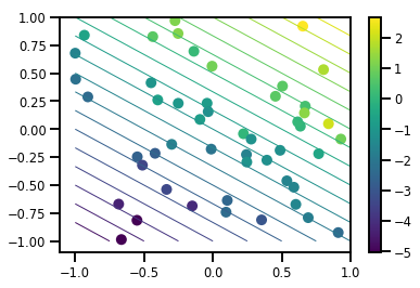
یک مجموعه داده تولید کنید

# Generate some data
def f(x, w):
  # Pad x with 1's so we can add bias via matmul
  x = tf.pad(x, [[1, 0], [0, 0]], constant_values=1)
  linop = tf.linalg.LinearOperatorFullMatrix(w[..., np.newaxis])
  result = linop.matmul(x, adjoint=True)
  return result[..., 0, :]

num_features = 2
num_examples = 50
noise_scale = .5
true_w = np.array([-1., 2., 3.])

xs = np.random.uniform(-1., 1., [num_features, num_examples])
ys = f(xs, true_w) + np.random.normal(0., noise_scale, size=num_examples)

# Visualize the data set
plt.scatter(*xs, c=ys, s=100, linewidths=0)

grid = np.meshgrid(*([np.linspace(-1, 1, 100)] * 2))
xs_grid = np.stack(grid, axis=0)
fs_grid = f(xs_grid.reshape([num_features, -1]), true_w)
fs_grid = np.reshape(fs_grid, [100, 100])
plt.colorbar()
plt.contour(xs_grid[0, ...], xs_grid[1, ...], fs_grid, 20, linewidths=1)
plt.show()

تابع log-prob مشترک ما را تعریف کنید

خلفی unnormalized نتیجه بسته شدن بیش از داده به شکل یک است برنامه جزئی از پروب ورود به سیستم مشترک.

# Define the joint_log_prob function, and our unnormalized posterior.
def joint_log_prob(w, x, y):
  # Our model in maths is
  #   w ~ MVN([0, 0, 0], diag([1, 1, 1]))
  #   y_i ~ Normal(w @ x_i, noise_scale),  i=1..N

  rv_w = tfd.MultivariateNormalDiag(
    loc=np.zeros(num_features + 1),
    scale_diag=np.ones(num_features + 1))

  rv_y = tfd.Normal(f(x, w), noise_scale)
  return (rv_w.log_prob(w) +
          tf.reduce_sum(rv_y.log_prob(y), axis=-1))

# Create our unnormalized target density by currying x and y from the joint.
def unnormalized_posterior(w):
  return joint_log_prob(w, xs, ys)

HMC TransitionKernel بسازید و sample_chain را فراخوانی کنید

# Create an HMC TransitionKernel
hmc_kernel = tfp.mcmc.HamiltonianMonteCarlo(
  target_log_prob_fn=unnormalized_posterior,
  step_size=np.float64(.1),
  num_leapfrog_steps=2)

# We wrap sample_chain in tf.function, telling TF to precompile a reusable
# computation graph, which will dramatically improve performance.
@tf.function
def run_chain(initial_state, num_results=1000, num_burnin_steps=500):
  return tfp.mcmc.sample_chain(
    num_results=num_results,
    num_burnin_steps=num_burnin_steps,
    current_state=initial_state,
    kernel=hmc_kernel,
    trace_fn=lambda current_state, kernel_results: kernel_results)

initial_state = np.zeros(num_features + 1)
samples, kernel_results = run_chain(initial_state)
print("Acceptance rate:", kernel_results.is_accepted.numpy().mean())

Acceptance rate: 0.915

این عالی نیست! ما می خواهیم نرخ پذیرش نزدیک به 0.65 باشد.

(نگاه کنید به "بهینه پوسته پوسته شدن برای مختلف کلانشهر-هیستینگز الگوریتم" ، رابرتز و روزنتال، 2001)

اندازه های گام تطبیقی

ما می توانیم HMC TransitionKernel ما در یک بسته بندی SimpleStepSizeAdaptation "متا هسته"، که برخی (اکتشافی و نه ساده) منطق برای انطباق اندازه گام شورای عالی رسانه ها در طول میسوزم اعمال خواهد شد. ما 80% از سوختن را برای تطبیق اندازه مرحله اختصاص می دهیم و سپس 20% باقیمانده را فقط به مخلوط کردن می دهیم.

# Apply a simple step size adaptation during burnin
@tf.function
def run_chain(initial_state, num_results=1000, num_burnin_steps=500):
  adaptive_kernel = tfp.mcmc.SimpleStepSizeAdaptation(
      hmc_kernel,
      num_adaptation_steps=int(.8 * num_burnin_steps),
      target_accept_prob=np.float64(.65))

  return tfp.mcmc.sample_chain(
    num_results=num_results,
    num_burnin_steps=num_burnin_steps,
    current_state=initial_state,
    kernel=adaptive_kernel,
    trace_fn=lambda cs, kr: kr)

samples, kernel_results = run_chain(
  initial_state=np.zeros(num_features+1))
print("Acceptance rate:", kernel_results.inner_results.is_accepted.numpy().mean())

Acceptance rate: 0.634

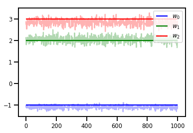
# Trace plots
colors = ['b', 'g', 'r']
for i in range(3):
  plt.plot(samples[:, i], c=colors[i], alpha=.3)
  plt.hlines(true_w[i], 0, 1000, zorder=4, color=colors[i], label="$w_{}$".format(i))
plt.legend(loc='upper right')
plt.show()

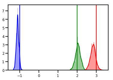
# Histogram of samples
for i in range(3):
  sns.distplot(samples[:, i], color=colors[i])
ymax = plt.ylim()[1]
for i in range(3):
  plt.vlines(true_w[i], 0, ymax, color=colors[i])
plt.ylim(0, ymax)
plt.show()

تشخیص

نمودارهای ردیابی خوب هستند، اما تشخیص بهتر است!

ابتدا باید چندین زنجیره را اجرا کنیم. این عنوان ساده به عنوان به دسته ای از initial_state تانسورها.

# Instead of a single set of initial w's, we create a batch of 8.
num_chains = 8
initial_state = np.zeros([num_chains, num_features + 1])

chains, kernel_results = run_chain(initial_state)

r_hat = tfp.mcmc.potential_scale_reduction(chains)
print("Acceptance rate:", kernel_results.inner_results.is_accepted.numpy().mean())
print("R-hat diagnostic (per latent variable):", r_hat.numpy())

Acceptance rate: 0.59175
R-hat diagnostic (per latent variable): [0.99998395 0.99932185 0.9997064 ]

نمونه برداری از مقیاس نویز

# Define the joint_log_prob function, and our unnormalized posterior.
def joint_log_prob(w, sigma, x, y):
  # Our model in maths is
  #   w ~ MVN([0, 0, 0], diag([1, 1, 1]))
  #   y_i ~ Normal(w @ x_i, noise_scale),  i=1..N

  rv_w = tfd.MultivariateNormalDiag(
    loc=np.zeros(num_features + 1),
    scale_diag=np.ones(num_features + 1))

  rv_sigma = tfd.LogNormal(np.float64(1.), np.float64(5.))

  rv_y = tfd.Normal(f(x, w), sigma[..., np.newaxis])
  return (rv_w.log_prob(w) +
          rv_sigma.log_prob(sigma) +
          tf.reduce_sum(rv_y.log_prob(y), axis=-1))

# Create our unnormalized target density by currying x and y from the joint.
def unnormalized_posterior(w, sigma):
  return joint_log_prob(w, sigma, xs, ys)


# Create an HMC TransitionKernel
hmc_kernel = tfp.mcmc.HamiltonianMonteCarlo(
  target_log_prob_fn=unnormalized_posterior,
  step_size=np.float64(.1),
  num_leapfrog_steps=4)



# Create a TransformedTransitionKernl
transformed_kernel = tfp.mcmc.TransformedTransitionKernel(
    inner_kernel=hmc_kernel,
    bijector=[tfb.Identity(),    # w
              tfb.Invert(tfb.Softplus())])   # sigma


# Apply a simple step size adaptation during burnin
@tf.function
def run_chain(initial_state, num_results=1000, num_burnin_steps=500):
  adaptive_kernel = tfp.mcmc.SimpleStepSizeAdaptation(
      transformed_kernel,
      num_adaptation_steps=int(.8 * num_burnin_steps),
      target_accept_prob=np.float64(.75))

  return tfp.mcmc.sample_chain(
    num_results=num_results,
    num_burnin_steps=num_burnin_steps,
    current_state=initial_state,
    kernel=adaptive_kernel,
    seed=(0, 1),
    trace_fn=lambda cs, kr: kr)


# Instead of a single set of initial w's, we create a batch of 8.
num_chains = 8
initial_state = [np.zeros([num_chains, num_features + 1]),
                 .54 * np.ones([num_chains], dtype=np.float64)]

chains, kernel_results = run_chain(initial_state)

r_hat = tfp.mcmc.potential_scale_reduction(chains)
print("Acceptance rate:", kernel_results.inner_results.inner_results.is_accepted.numpy().mean())
print("R-hat diagnostic (per w variable):", r_hat[0].numpy())
print("R-hat diagnostic (sigma):", r_hat[1].numpy())

Acceptance rate: 0.715875
R-hat diagnostic (per w variable): [1.0000073  1.00458208 1.00450512]
R-hat diagnostic (sigma): 1.0092056996149859

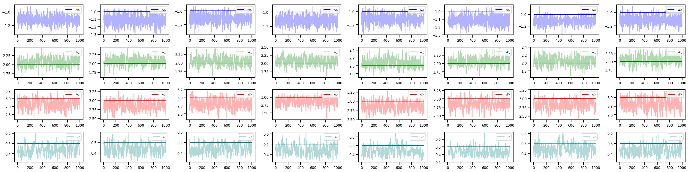
w_chains, sigma_chains = chains

# Trace plots of w (one of 8 chains)
colors = ['b', 'g', 'r', 'teal']
fig, axes = plt.subplots(4, num_chains, figsize=(4 * num_chains, 8))
for j in range(num_chains):
  for i in range(3):
    ax = axes[i][j]
    ax.plot(w_chains[:, j, i], c=colors[i], alpha=.3)
    ax.hlines(true_w[i], 0, 1000, zorder=4, color=colors[i], label="$w_{}$".format(i))
    ax.legend(loc='upper right')
  ax = axes[3][j]
  ax.plot(sigma_chains[:, j], alpha=.3, c=colors[3])
  ax.hlines(noise_scale, 0, 1000, zorder=4, color=colors[3], label=r"$\sigma$".format(i))
  ax.legend(loc='upper right')
fig.tight_layout()
plt.show()

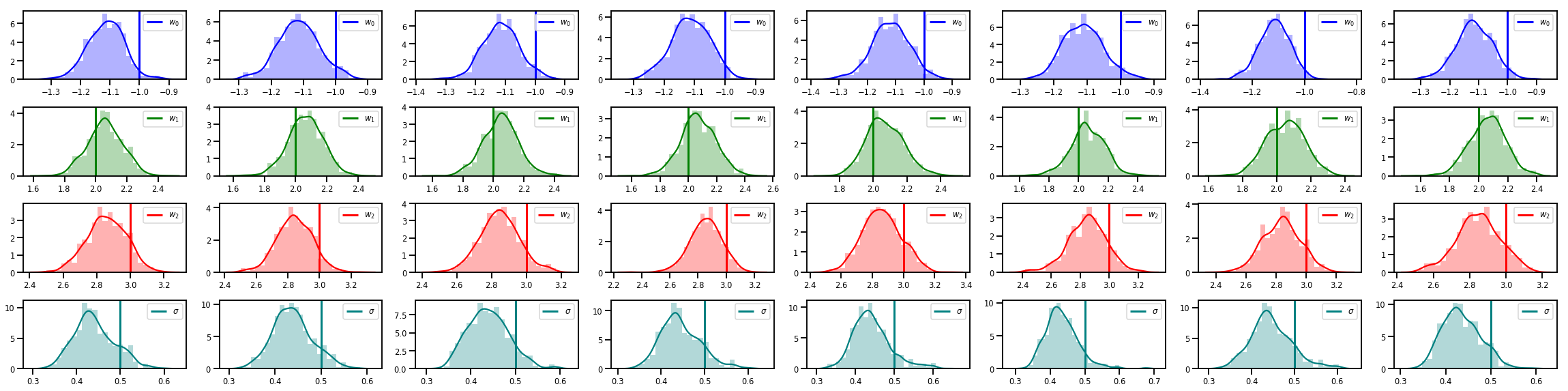
# Histogram of samples of w
fig, axes = plt.subplots(4, num_chains, figsize=(4 * num_chains, 8))
for j in range(num_chains):
  for i in range(3):
    ax = axes[i][j]
    sns.distplot(w_chains[:, j, i], color=colors[i], norm_hist=True, ax=ax, hist_kws={'alpha': .3})
  for i in range(3):
    ax = axes[i][j]
    ymax = ax.get_ylim()[1]
    ax.vlines(true_w[i], 0, ymax, color=colors[i], label="$w_{}$".format(i), linewidth=3)
    ax.set_ylim(0, ymax)
    ax.legend(loc='upper right')


  ax = axes[3][j]
  sns.distplot(sigma_chains[:, j], color=colors[3], norm_hist=True, ax=ax, hist_kws={'alpha': .3})
  ymax = ax.get_ylim()[1]
  ax.vlines(noise_scale, 0, ymax, color=colors[3], label=r"$\sigma$".format(i), linewidth=3)
  ax.set_ylim(0, ymax)
  ax.legend(loc='upper right')
fig.tight_layout()
plt.show()

خیلی بیشتر هم هست!

این پست ها و نمونه های جالب وبلاگ را بررسی کنید:

• سازه سری زمانی پشتیبانی وبلاگ COLAB
• لایه احتمالاتی Keras (ورودی: تانسور، خروجی: توزیع!) وبلاگ COLAB
  • یکی دیگر از لایه به عنوان مثال: VAEs وبلاگ COLAB
• گاوسی رگرسیون فرآیند COLAB و متغیر مکنون مدلسازی COLAB

نمونه های بیشتر و نوت بوک در GitHub ما در اینجا !