
| | |  مشاهده منبع در GitHub مشاهده منبع در GitHub | |
در این colab، ما رگرسیون فرآیند گاوسی را با استفاده از TensorFlow و TensorFlow Probability بررسی می کنیم. ما برخی از مشاهدات پر سر و صدا را از برخی عملکردهای شناخته شده تولید می کنیم و مدل های GP را با آن داده ها مطابقت می دهیم. سپس از GP خلفی نمونه برداری می کنیم و مقادیر تابع نمونه برداری شده را بر روی شبکه های حوزه آنها رسم می کنیم.
زمینه
اجازه دهید \(\mathcal{X}\) تواند هر مجموعه ای. یک Gaussian فرآیند (GP) مجموعه ای از متغیرهای تصادفی نمایه شده توسط است \(\mathcal{X}\) به طوری که اگر\(\{X_1, \ldots, X_n\} \subset \mathcal{X}\) هر زیر مجموعه ای متناهی است، چگالی حاشیه\(p(X_1 = x_1, \ldots, X_n = x_n)\) چند متغیره است گاوسی. هر توزیع گاوسی به طور کامل توسط لحظه های مرکزی اول و دوم آن (میانگین و کوواریانس) مشخص می شود و GP ها از این قاعده مستثنی نیستند. ما می توانیم یک GP کاملا از نظر میانگین آن تابع را مشخص \(\mu : \mathcal{X} \to \mathbb{R}\) و کوواریانس تابع\(k : \mathcal{X} \times \mathcal{X} \to \mathbb{R}\). بیشتر قدرت بیانی GP در انتخاب تابع کوواریانس محصور شده است. به دلایل مختلف، تابع کواریانس نیز به عنوان یک تابع هسته نامیده می شود. لازم است تنها به متقارن و مثبت قطعی (نگاه کنید به فصل 4 از راسموسن و ویلیامز ). در زیر از هسته کوواریانس ExponentiatedQuadratic استفاده می کنیم. شکل آن است
\[ k(x, x') := \sigma^2 \exp \left( \frac{\|x - x'\|^2}{\lambda^2} \right) \]
که در آن \(\sigma^2\) شده "دامنه" و به نام \(\lambda\) مقیاس طول است. پارامترهای هسته را می توان از طریق یک روش بهینه سازی حداکثر احتمال انتخاب کرد.
نمونه کامل از یک پزشک عمومی شامل مقدار واقعی تابع بیش از فضای کل\(\mathcal{X}\) و در عمل غیر عملی به درک این است؛ اغلب فرد مجموعه ای از نقاط را برای مشاهده نمونه انتخاب می کند و مقادیر تابع را در این نقاط ترسیم می کند. این با نمونه برداری از یک گاوسی چند متغیره مناسب (بعد محدود) به دست می آید.
توجه داشته باشید که طبق تعریف فوق، هر توزیع گاوسی چند متغیره محدود نیز یک فرآیند گاوسی است. معمولا، زمانی که یکی به یک پزشک عمومی اشاره دارد، آن است که به طور ضمنی مجموعه ای شاخص برخی \(\mathbb{R}^n\)و ما در واقع این فرض را در اینجا.
یکی از کاربردهای رایج فرآیندهای گاوسی در یادگیری ماشین، رگرسیون فرآیند گاوسی است. ایده این است که ما مایل به برآورد تابع ناشناخته مشاهدات پر سر و صدا داده \(\{y_1, \ldots, y_N\}\) از تابع در یک تعداد متناهی از نقاط \(\{x_1, \ldots x_N\}.\) ما یک فرایند مولد تصور
\[ \begin{align} f \sim \: & \textsf{GaussianProcess}\left( \text{mean_fn}=\mu(x), \text{covariance_fn}=k(x, x')\right) \\ y_i \sim \: & \textsf{Normal}\left( \text{loc}=f(x_i), \text{scale}=\sigma\right), i = 1, \ldots, N \end{align} \]
همانطور که در بالا ذکر شد، محاسبه تابع نمونه غیرممکن است، زیرا ما به مقدار آن در تعداد بی نهایت نقطه نیاز داریم. در عوض، یک نمونه محدود از یک گاوسی چند متغیره را در نظر می گیریم.
\[ \begin{gather} \begin{bmatrix} f(x_1) \\ \vdots \\ f(x_N) \end{bmatrix} \sim \textsf{MultivariateNormal} \left( \: \text{loc}= \begin{bmatrix} \mu(x_1) \\ \vdots \\ \mu(x_N) \end{bmatrix} \:,\: \text{scale}= \begin{bmatrix} k(x_1, x_1) & \cdots & k(x_1, x_N) \\ \vdots & \ddots & \vdots \\ k(x_N, x_1) & \cdots & k(x_N, x_N) \\ \end{bmatrix}^{1/2} \: \right) \end{gather} \\ y_i \sim \textsf{Normal} \left( \text{loc}=f(x_i), \text{scale}=\sigma \right) \]
توجه داشته باشید که توان \(\frac{1}{2}\) در ماتریس کوواریانس: این نشان دهنده یک تجزیه Cholesky. محاسبه Cholesky ضروری است زیرا MVN یک توزیع خانوادگی در مقیاس مکان است. متاسفانه تجزیه Cholesky محاسباتی گران است، گرفتن \(O(N^3)\) زمان و \(O(N^2)\) فضا. بسیاری از ادبیات عمومی پزشک معطوف به برخورد با این شارح کوچک به ظاهر بی ضرر است.
معمول است که تابع میانگین قبلی را ثابت و اغلب صفر در نظر بگیریم. همچنین، برخی از قراردادهای نمادی راحت هستند. اغلب می نویسد \(\mathbf{f}\) برای بردار متناهی از مقادیر تابع نمونه برداری شد. تعدادی از نمادهای جالب برای ماتریس کواریانس ناشی از استفاده از استفاده \(k\) به جفت ورودی. زیر (Quiñonero-کاندلا، 2005) ، توجه داشته باشید که اجزای ماتریس کواریانس مقادیر تابع در نقاط ورودی خاص می باشد. بنابراین ما می توانیم ماتریس کوواریانس است که به عنوان \(K_{AB}\)که در آن \(A\) و \(B\) برخی از شاخص های از مجموعه ای از مقادیر تابع در امتداد ابعاد ماتریس داده شده است.
به عنوان مثال، با توجه به داده های مشاهده شده \((\mathbf{x}, \mathbf{y})\) با ارزش کارکرد پنهان ضمنی \(\mathbf{f}\)، ما می توانیم ارسال
\[ K_{\mathbf{f},\mathbf{f} } = \begin{bmatrix} k(x_1, x_1) & \cdots & k(x_1, x_N) \\ \vdots & \ddots & \vdots \\ k(x_N, x_1) & \cdots & k(x_N, x_N) \\ \end{bmatrix} \]
به طور مشابه، میتوانیم مجموعهای از ورودیها را با هم ترکیب کنیم
\[ K_{\mathbf{f},*} = \begin{bmatrix} k(x_1, x^*_1) & \cdots & k(x_1, x^*_T) \\ \vdots & \ddots & \vdots \\ k(x_N, x^*_1) & \cdots & k(x_N, x^*_T) \\ \end{bmatrix} \]
که در آن ما فرض وجود دارد \(N\) ورودی آموزش و \(T\) ورودی آزمون. فرآیند تولیدی فوق ممکن است به صورت فشرده نوشته شود
\[ \begin{align} \mathbf{f} \sim \: & \textsf{MultivariateNormal} \left( \text{loc}=\mathbf{0}, \text{scale}=K_{\mathbf{f},\mathbf{f} }^{1/2} \right) \\ y_i \sim \: & \textsf{Normal} \left( \text{loc}=f_i, \text{scale}=\sigma \right), i = 1, \ldots, N \end{align} \]
این عملیات نمونه برداری در خط اول بازده یک مجموعه متناهی از \(N\) مقادیر تابع از یک Gaussian چند متغیره - و نه یک تابع کل همانطور که در بالا نماد GP قرعه کشی. خط دوم توصیف مجموعه ای از \(N\) تساوی از Gaussians تک متغیره در مقادیر عملکرد های مختلف و با حداقل سر و صدا ثابت مشاهده \(\sigma^2\).
با در نظر گرفتن مدل تولیدی فوق، میتوانیم مشکل استنتاج پسین را در نظر بگیریم. این یک توزیع پسینی را بر روی مقادیر تابع در مجموعه جدیدی از نقاط آزمایش، مشروط به دادههای نویز مشاهده شده از فرآیند بالا، ایجاد میکند.
با نماد بالا در محل، ما فشرده می توانید ارسال توزیع پیش بینی خلفی بر سر آینده (پر سر و صدا) مشاهدات در ورودی ها و داده های آموزشی به شرح زیر است (برای جزئیات بیشتر، نگاه کنید §2.2 مربوط مشروط راسموسن و ویلیامز ).
\[ \mathbf{y}^* \mid \mathbf{x}^*, \mathbf{x}, \mathbf{y} \sim \textsf{Normal} \left( \text{loc}=\mathbf{\mu}^*, \text{scale}=(\Sigma^*)^{1/2} \right), \]
جایی که
\[ \mathbf{\mu}^* = K_{*,\mathbf{f} }\left(K_{\mathbf{f},\mathbf{f} } + \sigma^2 I \right)^{-1} \mathbf{y} \]
و
\[ \Sigma^* = K_{*,*} - K_{*,\mathbf{f} } \left(K_{\mathbf{f},\mathbf{f} } + \sigma^2 I \right)^{-1} K_{\mathbf{f},*} \]
واردات
import time

import numpy as np
import matplotlib.pyplot as plt
import tensorflow.compat.v2 as tf
import tensorflow_probability as tfp
tfb = tfp.bijectors
tfd = tfp.distributions
tfk = tfp.math.psd_kernels
tf.enable_v2_behavior()

from mpl_toolkits.mplot3d import Axes3D
%pylab inline
# Configure plot defaults
plt.rcParams['axes.facecolor'] = 'white'
plt.rcParams['grid.color'] = '#666666'
%config InlineBackend.figure_format = 'png'
Populating the interactive namespace from numpy and matplotlib
مثال: رگرسیون دقیق GP در داده های سینوسی نویزدار
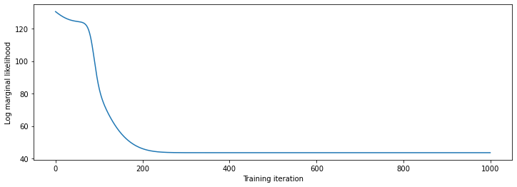
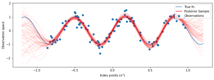
در اینجا ما داده های آموزشی را از یک سینوسی پر سر و صدا تولید می کنیم، سپس دسته ای از منحنی ها را از مدل رگرسیون GP نمونه برداری می کنیم. ما با استفاده از آدم برای بهینه سازی hyperparameters هسته (ما احتمال ورود منفی داده تحت قبل به حداقل رساندن). منحنی آموزش را رسم می کنیم و به دنبال آن تابع واقعی و نمونه های خلفی را نشان می دهیم.
def sinusoid(x):
  return np.sin(3 * np.pi * x[..., 0])

def generate_1d_data(num_training_points, observation_noise_variance):
  """Generate noisy sinusoidal observations at a random set of points.

  Returns:
     observation_index_points, observations
  """
  index_points_ = np.random.uniform(-1., 1., (num_training_points, 1))
  index_points_ = index_points_.astype(np.float64)
  # y = f(x) + noise
  observations_ = (sinusoid(index_points_) +
                   np.random.normal(loc=0,
                                    scale=np.sqrt(observation_noise_variance),
                                    size=(num_training_points)))
  return index_points_, observations_
# Generate training data with a known noise level (we'll later try to recover
# this value from the data).
NUM_TRAINING_POINTS = 100
observation_index_points_, observations_ = generate_1d_data(
    num_training_points=NUM_TRAINING_POINTS,
    observation_noise_variance=.1)
ما priors در hyperparameters هسته قرار داده، و ارسال به توزیع مشترک از hyperparameters و داده های مشاهده شده با استفاده از tfd.JointDistributionNamed .
def build_gp(amplitude, length_scale, observation_noise_variance):
  """Defines the conditional dist. of GP outputs, given kernel parameters."""

  # Create the covariance kernel, which will be shared between the prior (which we
  # use for maximum likelihood training) and the posterior (which we use for
  # posterior predictive sampling)
  kernel = tfk.ExponentiatedQuadratic(amplitude, length_scale)

  # Create the GP prior distribution, which we will use to train the model
  # parameters.
  return tfd.GaussianProcess(
      kernel=kernel,
      index_points=observation_index_points_,
      observation_noise_variance=observation_noise_variance)

gp_joint_model = tfd.JointDistributionNamed({
    'amplitude': tfd.LogNormal(loc=0., scale=np.float64(1.)),
    'length_scale': tfd.LogNormal(loc=0., scale=np.float64(1.)),
    'observation_noise_variance': tfd.LogNormal(loc=0., scale=np.float64(1.)),
    'observations': build_gp,
})
میتوانیم با تأیید اینکه میتوانیم از نمونههای قبلی نمونهبرداری کنیم، اجرای خود را بررسی کنیم و چگالی لگ یک نمونه را محاسبه کنیم.
x = gp_joint_model.sample()
lp = gp_joint_model.log_prob(x)

print("sampled {}".format(x))
print("log_prob of sample: {}".format(lp))
sampled {'observation_noise_variance': <tf.Tensor: shape=(), dtype=float64, numpy=2.067952217184325>, 'length_scale': <tf.Tensor: shape=(), dtype=float64, numpy=1.154435715487831>, 'amplitude': <tf.Tensor: shape=(), dtype=float64, numpy=5.383850737703549>, 'observations': <tf.Tensor: shape=(100,), dtype=float64, numpy=
array([-2.37070577, -2.05363838, -0.95152824,  3.73509388, -0.2912646 ,
        0.46112342, -1.98018513, -2.10295857, -1.33589756, -2.23027226,
       -2.25081374, -0.89450835, -2.54196452,  1.46621647,  2.32016193,
        5.82399989,  2.27241034, -0.67523432, -1.89150197, -1.39834474,
       -2.33954116,  0.7785609 , -1.42763627, -0.57389025, -0.18226098,
       -3.45098732,  0.27986652, -3.64532398, -1.28635204, -2.42362875,
        0.01107288, -2.53222176, -2.0886136 , -5.54047694, -2.18389607,
       -1.11665628, -3.07161217, -2.06070336, -0.84464262,  1.29238438,
       -0.64973999, -2.63805504, -3.93317576,  0.65546645,  2.24721181,
       -0.73403676,  5.31628298, -1.2208384 ,  4.77782252, -1.42978168,
       -3.3089274 ,  3.25370494,  3.02117591, -1.54862932, -1.07360811,
        1.2004856 , -4.3017773 , -4.95787789, -1.95245901, -2.15960839,
       -3.78592731, -1.74096185,  3.54891595,  0.56294143,  1.15288455,
       -0.77323696,  2.34430694, -1.05302007, -0.7514684 , -0.98321063,
       -3.01300144, -3.00033274,  0.44200837,  0.45060886, -1.84497318,
       -1.89616746, -2.15647664, -2.65672581, -3.65493379,  1.70923375,
       -3.88695218, -0.05151283,  4.51906677, -2.28117003,  3.03032793,
       -1.47713194, -0.35625273,  3.73501587, -2.09328047, -0.60665614,
       -0.78177188, -0.67298545,  2.97436033, -0.29407932,  2.98482427,
       -1.54951178,  2.79206821,  4.2225733 ,  2.56265198,  2.80373284])>}
log_prob of sample: -194.96442183797524
حالا بیایید برای یافتن مقادیر پارامتر با بالاترین احتمال پسین بهینه سازی کنیم. برای هر پارامتر یک متغیر تعریف می کنیم و مقادیر آنها را مثبت می کنیم.
# Create the trainable model parameters, which we'll subsequently optimize.
# Note that we constrain them to be strictly positive.

constrain_positive = tfb.Shift(np.finfo(np.float64).tiny)(tfb.Exp())

amplitude_var = tfp.util.TransformedVariable(
    initial_value=1.,
    bijector=constrain_positive,
    name='amplitude',
    dtype=np.float64)

length_scale_var = tfp.util.TransformedVariable(
    initial_value=1.,
    bijector=constrain_positive,
    name='length_scale',
    dtype=np.float64)

observation_noise_variance_var = tfp.util.TransformedVariable(
    initial_value=1.,
    bijector=constrain_positive,
    name='observation_noise_variance_var',
    dtype=np.float64)

trainable_variables = [v.trainable_variables[0] for v in
                       [amplitude_var,
                       length_scale_var,
                       observation_noise_variance_var]]
مشروط کردن مدل در داده های مشاهده شده ما، ما به یک تعریف target_log_prob تابع، که (هنوز هم به استنباط می شود) hyperparameters هسته طول می کشد.
def target_log_prob(amplitude, length_scale, observation_noise_variance):
  return gp_joint_model.log_prob({
      'amplitude': amplitude,
      'length_scale': length_scale,
      'observation_noise_variance': observation_noise_variance,
      'observations': observations_
  })
# Now we optimize the model parameters.
num_iters = 1000
optimizer = tf.optimizers.Adam(learning_rate=.01)

# Use `tf.function` to trace the loss for more efficient evaluation.
@tf.function(autograph=False, jit_compile=False)
def train_model():
  with tf.GradientTape() as tape:
    loss = -target_log_prob(amplitude_var, length_scale_var,
                            observation_noise_variance_var)
  grads = tape.gradient(loss, trainable_variables)
  optimizer.apply_gradients(zip(grads, trainable_variables))
  return loss

# Store the likelihood values during training, so we can plot the progress
lls_ = np.zeros(num_iters, np.float64)
for i in range(num_iters):
  loss = train_model()
  lls_[i] = loss

print('Trained parameters:')
print('amplitude: {}'.format(amplitude_var._value().numpy()))
print('length_scale: {}'.format(length_scale_var._value().numpy()))
print('observation_noise_variance: {}'.format(observation_noise_variance_var._value().numpy()))
Trained parameters:
amplitude: 0.9176153445125278
length_scale: 0.18444082442910079
observation_noise_variance: 0.0880273312850989
# Plot the loss evolution
plt.figure(figsize=(12, 4))
plt.plot(lls_)
plt.xlabel("Training iteration")
plt.ylabel("Log marginal likelihood")
plt.show()
# Having trained the model, we'd like to sample from the posterior conditioned
# on observations. We'd like the samples to be at points other than the training
# inputs.
predictive_index_points_ = np.linspace(-1.2, 1.2, 200, dtype=np.float64)
# Reshape to [200, 1] -- 1 is the dimensionality of the feature space.
predictive_index_points_ = predictive_index_points_[..., np.newaxis]

optimized_kernel = tfk.ExponentiatedQuadratic(amplitude_var, length_scale_var)
gprm = tfd.GaussianProcessRegressionModel(
    kernel=optimized_kernel,
    index_points=predictive_index_points_,
    observation_index_points=observation_index_points_,
    observations=observations_,
    observation_noise_variance=observation_noise_variance_var,
    predictive_noise_variance=0.)

# Create op to draw  50 independent samples, each of which is a *joint* draw
# from the posterior at the predictive_index_points_. Since we have 200 input
# locations as defined above, this posterior distribution over corresponding
# function values is a 200-dimensional multivariate Gaussian distribution!
num_samples = 50
samples = gprm.sample(num_samples)
# Plot the true function, observations, and posterior samples.
plt.figure(figsize=(12, 4))
plt.plot(predictive_index_points_, sinusoid(predictive_index_points_),
         label='True fn')
plt.scatter(observation_index_points_[:, 0], observations_,
            label='Observations')
for i in range(num_samples):
  plt.plot(predictive_index_points_, samples[i, :], c='r', alpha=.1,
           label='Posterior Sample' if i == 0 else None)
leg = plt.legend(loc='upper right')
for lh in leg.legendHandles:
    lh.set_alpha(1)
plt.xlabel(r"Index points ($\mathbb{R}^1$)")
plt.ylabel("Observation space")
plt.show()
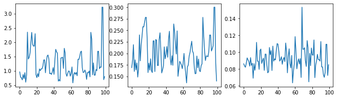
حاشیه سازی هایپرپارامترها با HMC
به جای بهینه سازی فراپارامترها، بیایید سعی کنیم آنها را با مونت کارلو همیلتونی ادغام کنیم. با توجه به مشاهدات، ابتدا یک نمونهگر را تعریف کرده و اجرا میکنیم تا تقریباً از توزیع خلفی روی فراپارامترهای هسته ترسیم شود.
num_results = 100
num_burnin_steps = 50

sampler = tfp.mcmc.TransformedTransitionKernel(
    tfp.mcmc.NoUTurnSampler(
        target_log_prob_fn=target_log_prob,
        step_size=tf.cast(0.1, tf.float64)),
    bijector=[constrain_positive, constrain_positive, constrain_positive])

adaptive_sampler = tfp.mcmc.DualAveragingStepSizeAdaptation(
    inner_kernel=sampler,
    num_adaptation_steps=int(0.8 * num_burnin_steps),
    target_accept_prob=tf.cast(0.75, tf.float64))

initial_state = [tf.cast(x, tf.float64) for x in [1., 1., 1.]]
# Speed up sampling by tracing with `tf.function`.
@tf.function(autograph=False, jit_compile=False)
def do_sampling():
  return tfp.mcmc.sample_chain(
      kernel=adaptive_sampler,
      current_state=initial_state,
      num_results=num_results,
      num_burnin_steps=num_burnin_steps,
      trace_fn=lambda current_state, kernel_results: kernel_results)

t0 = time.time()
samples, kernel_results = do_sampling()
t1 = time.time()
print("Inference ran in {:.2f}s.".format(t1-t0))
Inference ran in 9.00s.
بیایید با بررسی ردیابی هایپرپارامتر، نمونه گیر را بررسی کنیم.
(amplitude_samples,
 length_scale_samples,
 observation_noise_variance_samples) = samples

f = plt.figure(figsize=[15, 3])
for i, s in enumerate(samples):
  ax = f.add_subplot(1, len(samples) + 1, i + 1)
  ax.plot(s)
حالا به جای ساخت یک GP تنها با hyperparameters بهینه سازی شده، ما توزیع پیش بینی خلفی به عنوان ترکیبی از پزشکان، هر تعریف شده توسط یک نمونه از توزیع خلفی بیش از hyperparameters ساخت. این تقریباً با پارامترهای خلفی از طریق نمونهبرداری مونت کارلو ادغام میشود تا توزیع پیشبینی حاشیهای را در مکانهای مشاهده نشده محاسبه کند.
# The sampled hyperparams have a leading batch dimension, `[num_results, ...]`,
# so they construct a *batch* of kernels.
batch_of_posterior_kernels = tfk.ExponentiatedQuadratic(
    amplitude_samples, length_scale_samples)

# The batch of kernels creates a batch of GP predictive models, one for each
# posterior sample.
batch_gprm = tfd.GaussianProcessRegressionModel(
    kernel=batch_of_posterior_kernels,
    index_points=predictive_index_points_,
    observation_index_points=observation_index_points_,
    observations=observations_,
    observation_noise_variance=observation_noise_variance_samples,
    predictive_noise_variance=0.)

# To construct the marginal predictive distribution, we average with uniform
# weight over the posterior samples.
predictive_gprm = tfd.MixtureSameFamily(
    mixture_distribution=tfd.Categorical(logits=tf.zeros([num_results])),
    components_distribution=batch_gprm)

num_samples = 50
samples = predictive_gprm.sample(num_samples)
# Plot the true function, observations, and posterior samples.
plt.figure(figsize=(12, 4))
plt.plot(predictive_index_points_, sinusoid(predictive_index_points_),
         label='True fn')
plt.scatter(observation_index_points_[:, 0], observations_,
            label='Observations')
for i in range(num_samples):
  plt.plot(predictive_index_points_, samples[i, :], c='r', alpha=.1,
           label='Posterior Sample' if i == 0 else None)
leg = plt.legend(loc='upper right')
for lh in leg.legendHandles:
    lh.set_alpha(1)
plt.xlabel(r"Index points ($\mathbb{R}^1$)")
plt.ylabel("Observation space")
plt.show()
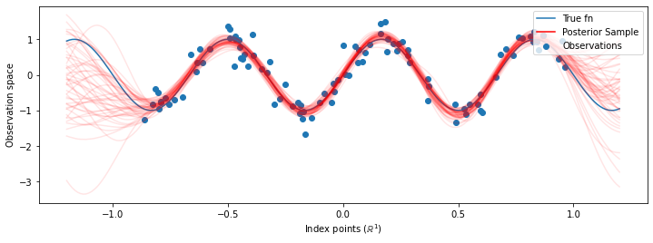
اگرچه تفاوتها در این مورد ظریف هستند، به طور کلی، ما انتظار داریم که توزیع پیشبینیکننده پسین بهتر تعمیم یابد (احتمال بیشتری به دادههای نگهداشتهشده بدهد) نسبت به استفاده از محتملترین پارامترها همانطور که در بالا انجام دادیم.