
| | |  مشاهده منبع در GitHub مشاهده منبع در GitHub | |
استنتاج متغیر (VI) استنتاج بیزی تقریبی را به عنوان یک مسئله بهینهسازی ارائه میکند و به دنبال توزیع خلفی «جانشین» است که واگرایی KL را با پسین واقعی به حداقل میرساند. VI مبتنی بر گرادیان اغلب سریعتر از روشهای MCMC است، به طور طبیعی با بهینهسازی پارامترهای مدل ترکیب میشود، و حد پایینتری در شواهد مدل ارائه میکند که میتواند مستقیماً برای مقایسه مدل، تشخیص همگرایی، و استنتاج قابل ترکیب استفاده شود.
TensorFlow Probability ابزارهایی را برای VI سریع، انعطاف پذیر و مقیاس پذیر ارائه می دهد که به طور طبیعی در پشته TFP قرار می گیرند. این ابزارها ساخت جانشینهای خلفی را با ساختارهای کوواریانس ناشی از تبدیلهای خطی یا عادیسازی جریانها امکانپذیر میسازند.
VI می توان برای برآورد بیزی فواصل معتبر برای پارامترهای یک مدل رگرسیون برآورد اثرات درمان های مختلف و یا ویژگی های مشاهده شده در نتیجه از علاقه. فواصل معتبر، مقادیر یک پارامتر مشاهده نشده را با احتمال معینی، با توجه به توزیع پسین پارامتر مشروط بر داده های مشاهده شده و فرضی بر توزیع قبلی پارامتر، محدود می کنند.
در این COLAB، ما نشان دهد که چگونه به استفاده از VI برای به دست آوردن فواصل معتبر برای پارامترهای یک بیزی مدل رگرسیون خطی برای میزان رادون اندازه گیری در خانه (با استفاده از Gelman و همکاران (2007) رادون مجموعه داده. . دیدن نمونه های مشابه در استن). ما نشان دهد که چگونه بهره وری کل عوامل JointDistribution با ترکیب bijectors به ساخت و مناسب دو نوع posteriors جانشین رسا:
- یک توزیع نرمال استاندارد که توسط یک ماتریس بلوکی تبدیل شده است. ماتریس ممکن است منعکس کننده استقلال در میان برخی از مؤلفه های پسین و وابستگی در میان سایرین باشد، که فرض یک میدان متوسط یا کوواریانس کامل خلفی را تسهیل می کند.
- پیچیده تر، با ظرفیت بالاتر معکوس جریان خود کاهشی .
خلفی های جایگزین آموزش داده شده و با نتایج حاصل از خط پایه خلفی جانشین میانگین میدان، و همچنین نمونه های حقیقت زمینی از همیلتونی مونت کارلو مقایسه می شوند.
مروری بر استنتاج متغیر بیزی
فرض کنید ما این کار زیر مولد، که در آن \(\theta\) نشان دهنده پارامترهای تصادفی، \(\omega\) نشان دهنده پارامترهای قطعی و \(x_i\) ویژگی های هستند و \(y_i\) مقادیر هدف برای \(i=1,\ldots,n\) مشاهده نقاط داده میشود: \ begin {چین } &\theta \sim r(\Theta) && \text{(Prior)}\ &\text{برای } i = 1 \ldots n: \nonumber \ &\quad y_i \sim p(Y_i|x_i, \theta ، \ امگا) && \ متن {(احتمال)} \ پایان {} چین
سپس VI با این ویژگی مشخص می شود: $\newcommand{\E}{\operatorname{\mathbb{E} } \newcommand{\K}{\operatorname{\mathbb{K} } } \newcommand{\defeq}{\overset {\tiny\text{def} }{=} } \DeclareMathOperator*{\argmin}{arg\,min}$
\ {آغاز تراز} - \ ورود به سیستم P ({y_i} _i ^ N | {x_i به} _i ^ N، \ امگا) و \ defeq - \ ورود \ INT \ textrm {D} \ تتا \ r و (\ theta) از \ prod_i^np(y_i|x_i،\theta، \omega) && \text{(انتگرال واقعاً سخت)} \ &= -\log \int \textrm{d}\theta\, q(\theta) \frac{1 }{q(\theta)} r(\theta) \prod_i^np(y_i|x_i،\theta، \omega) && \text{(ضرب در 1)}\ &\le - \int \textrm{d} \ تتا \، Q (\ theta) از \ ورود که \ frac {R (\ theta) از \ prod_i ^ NP (y_i | X من، \ تتا، \ امگا)} {Q (\ theta) از} && \ متن {(نابرابری ینسن )} \ & \ defeq \ E {Q (\ تتا)} [- \ ورود P (y_i | x_i به، \ تتا، \ امگا)] + \ K [Q (\ تتا)، R (\ تتا)] \ & \ defeq \text{expected negative log likelihood"} + \ متن {تنظیم کننده KL"} \ پایان {} چین
(از نظر فنی ما در حال فرض \(q\) است کاملا پیوسته با توجه به \(r\)همچنین نگاه کنید به، نابرابری ینسن .)
از آنجایی که کران برای همه q برقرار است، واضح است که برای:
\[q^*,w^* = \argmin_{q \in \mathcal{Q},\omega\in\mathbb{R}^d} \left\{ \sum_i^n\E_{q(\Theta)}\left[ -\log p(y_i|x_i,\Theta, \omega) \right] + \K[q(\Theta), r(\Theta)] \right\}\]
با توجه به اصطلاحات، ما تماس می گیریم
- \(q^*\) به "خلفی جانشین،" و،
- \(\mathcal{Q}\) "خانواده قائم مقام."
\(\omega^*\) نشان دهنده ارزش حداکثر احتمال از پارامترهای قطعی در از دست دادن VI. مشاهده این بررسی برای اطلاعات بیشتر بر استنتاج تغییرات.
مثال: رگرسیون خطی سلسله مراتبی بیزی بر روی اندازه گیری های رادون
رادون یک گاز رادیواکتیو است که از طریق نقاط تماس با زمین وارد خانه ها می شود. این یک ماده سرطان زا است که علت اصلی سرطان ریه در افراد غیر سیگاری است. سطوح رادون از خانواده ای به خانه دیگر بسیار متفاوت است.
EPA مطالعه ای در مورد سطوح رادون در 80000 خانه انجام داد. دو پیش بینی کننده مهم عبارتند از:
- طبقه ای که اندازه گیری روی آن انجام شده است (رادون در زیرزمین بیشتر است)
- سطح اورانیوم شهرستان (همبستگی مثبت با سطح رادون)
پیش بینی سطح رادون در خانه های گروه بندی شده توسط شهرستان یک مشکل کلاسیک در بیزی مدل سازی سلسله مراتبی، معرفی شده توسط است Gelman و هیل (2006) . ما یک مدل خطی سلسله مراتبی برای پیشبینی اندازهگیری رادون در خانهها خواهیم ساخت، که در آن سلسله مراتب، گروهبندی خانهها بر اساس شهرستان است. ما علاقه مند به فواصل معتبر برای تأثیر مکان (شهرستان) بر سطح رادون خانه ها در مینه سوتا هستیم. به منظور جداسازی این اثر، اثرات کف و سطح اورانیوم نیز در مدل گنجانده شده است. علاوه بر این، ما یک اثر زمینهای مربوط به میانگین طبقهای که اندازهگیری روی آن انجام شده است، به تفکیک شهرستان در نظر میگیریم، بهطوریکه اگر بین شهرستانهای طبقهای که اندازهگیریها در آن انجام شده، تفاوت وجود داشته باشد، این به اثر شهرستان نسبت داده نمیشود.
pip3 install -q tf-nightly tfp-nightly
import matplotlib.pyplot as plt
import numpy as np
import seaborn as sns
import tensorflow as tf
import tensorflow_datasets as tfds
import tensorflow_probability as tfp
import warnings

tfd = tfp.distributions
tfb = tfp.bijectors

plt.rcParams['figure.facecolor'] = '1.'
# Load the Radon dataset from `tensorflow_datasets` and filter to data from
# Minnesota.
dataset = tfds.as_numpy(
    tfds.load('radon', split='train').filter(
        lambda x: x['features']['state'] == 'MN').batch(10**9))

# Dependent variable: Radon measurements by house.
dataset = next(iter(dataset))
radon_measurement = dataset['activity'].astype(np.float32)
radon_measurement[radon_measurement <= 0.] = 0.1
log_radon = np.log(radon_measurement)

# Measured uranium concentrations in surrounding soil.
uranium_measurement = dataset['features']['Uppm'].astype(np.float32)
log_uranium = np.log(uranium_measurement)

# County indicator.
county_strings = dataset['features']['county'].astype('U13')
unique_counties, county = np.unique(county_strings, return_inverse=True)
county = county.astype(np.int32)
num_counties = unique_counties.size

# Floor on which the measurement was taken.
floor_of_house = dataset['features']['floor'].astype(np.int32)

# Average floor by county (contextual effect).
county_mean_floor = []
for i in range(num_counties):
  county_mean_floor.append(floor_of_house[county == i].mean())
county_mean_floor = np.array(county_mean_floor, dtype=log_radon.dtype)
floor_by_county = county_mean_floor[county]
مدل رگرسیون به صورت زیر مشخص می شود:
\(\newcommand{\Normal}{\operatorname{\sf Normal} }\)\ {آغاز تراز} و \ متن {uranium_weight} \ سیم کارت \ عادی (0، 1) \ & \ متن {county_floor_weight} \ سیم کارت \ عادی (0، 1) \ & \ متن {برای} J = 1 \ ldots \text{num_counties}:\ &\quad \text{county_effect}_j \sim \Normal (0, \sigma_c)\ &\text{برای } i = 1\ldots n:\ &\quad \mu_i = ( \ و \ چهار \ چهار \ متن {تعصب} \ & \ چهار \ چهار + \ متن {اثر شهرستان} {\ متن {شهرستان} _i} \ & \ چهار \ چهار + \ متن {log_uranium} _i \ بار \ متن {uranium_weight } \ & \ چهار \ چهار + \ متن {floor_of_house} _i \ بار \ متن {floor_weight} \ & \ چهار \ چهار + \ متن {شهرستان floor_by} {\ متن {شهرستان} _i} \ بار \ متن {county_floor_weight}) \ & \ چهار \ متن {log_radon} _i \ سیم کارت \ عادی (\ mu_i، \ sigma_y) \ پایان {چین} که در آن \(i\) شاخص مشاهدات و \(\text{county}_i\) است شهرستان که در آن \(i\)هفتم مشاهده بود گرفته شده.
ما از یک اثر تصادفی در سطح شهرستان برای ثبت تغییرات جغرافیایی استفاده می کنیم. پارامترهای uranium_weight و county_floor_weight می احتمالاتی مدل، و floor_weight و ثابت bias قطعی است. این انتخابهای مدلسازی تا حد زیادی دلخواه هستند و به منظور نشان دادن VI بر روی یک مدل احتمالی با پیچیدگی معقول ساخته شدهاند. برای بحث دقیق تر از مدل سازی چند سطحی با اثرات ثابت و تصادفی در بهره وری کل عوامل، با استفاده از مجموعه داده رادون، و چند مدل سازی پرایمر و اتصالات مختلط اثرات خطی تعمیم مدل با استفاده از تغییرات استنتاج .
# Create variables for fixed effects.
floor_weight = tf.Variable(0.)
bias = tf.Variable(0.)

# Variables for scale parameters.
log_radon_scale = tfp.util.TransformedVariable(1., tfb.Exp())
county_effect_scale = tfp.util.TransformedVariable(1., tfb.Exp())

# Define the probabilistic graphical model as a JointDistribution.
@tfd.JointDistributionCoroutineAutoBatched
def model():
  uranium_weight = yield tfd.Normal(0., scale=1., name='uranium_weight')
  county_floor_weight = yield tfd.Normal(
      0., scale=1., name='county_floor_weight')
  county_effect = yield tfd.Sample(
      tfd.Normal(0., scale=county_effect_scale),
      sample_shape=[num_counties], name='county_effect')
  yield tfd.Normal(
      loc=(log_uranium * uranium_weight + floor_of_house* floor_weight
           + floor_by_county * county_floor_weight
           + tf.gather(county_effect, county, axis=-1)
           + bias),
      scale=log_radon_scale[..., tf.newaxis],
      name='log_radon')

# Pin the observed `log_radon` values to model the un-normalized posterior.
target_model = model.experimental_pin(log_radon=log_radon)
خلفی جانشین بیانگر
در مرحله بعد، توزیع های خلفی اثرات تصادفی را با استفاده از VI با دو نوع مختلف جانشین پسین تخمین می زنیم:
- یک توزیع نرمال چند متغیره محدود، با ساختار کوواریانس ناشی از یک تبدیل ماتریس بلوکی.
- توزیع استاندارد نرمال چند متغیره تبدیل توسط یک معکوس خودرگرسیو جریان ، که پس از تقسیم و بازسازی برای مطابقت با حمایت از خلفی.
چند متغیره نرمال جانشین خلفی
برای ساخت این جانشین خلفی، از یک عملگر خطی قابل آموزش برای القای همبستگی بین اجزای خلفی استفاده میشود.
# Determine the `event_shape` of the posterior, and calculate the size of each
# `event_shape` component. These determine the sizes of the components of the
# underlying standard Normal distribution, and the dimensions of the blocks in
# the blockwise matrix transformation.
event_shape = target_model.event_shape_tensor()
flat_event_shape = tf.nest.flatten(event_shape)
flat_event_size = tf.nest.map_structure(tf.reduce_prod, flat_event_shape)

# The `event_space_bijector` maps unconstrained values (in R^n) to the support
# of the prior -- we'll need this at the end to constrain Multivariate Normal
# samples to the prior's support.
event_space_bijector = target_model.experimental_default_event_space_bijector()
ساخت یک JointDistribution با اجزای عادی استاندارد برداری مقدار، با اندازه های تعیین شده توسط اجزای قبل مربوطه. مولفه ها باید بردار باشند تا بتوانند توسط عملگر خطی تبدیل شوند.
base_standard_dist = tfd.JointDistributionSequential(
      [tfd.Sample(tfd.Normal(0., 1.), s) for s in flat_event_size])
یک عملگر خطی مثلثی پایین تر قابل آموزش بسازید. ما آن را به توزیع عادی استاندارد اعمال می کنیم تا یک تبدیل ماتریس بلوکی (قابل آموزش) را پیاده سازی کنیم و ساختار همبستگی قسمت خلفی را القا کنیم.
در اپراتور blockwise خطی، بلوک های کامل ماتریس کواریانس نشان دهنده تربیت شدنی کامل بین دو مولفه از خلفی، در حالی که یک بلوک از صفر (یا None ) بیان استقلال. بلوک های روی مورب یا ماتریس های مثلثی پایین یا مورب هستند، به طوری که کل ساختار بلوک نشان دهنده یک ماتریس مثلث پایین تر است.
اعمال این بیژکتور به توزیع پایه منجر به توزیع نرمال چند متغیره با میانگین 0 و کوواریانس (با عامل کلسکی) برابر با ماتریس بلوک مثلثی پایین می شود.
operators = (
    (tf.linalg.LinearOperatorDiag,),  # Variance of uranium weight (scalar).
    (tf.linalg.LinearOperatorFullMatrix,  # Covariance between uranium and floor-by-county weights.
     tf.linalg.LinearOperatorDiag),  # Variance of floor-by-county weight (scalar).
    (None,  # Independence between uranium weight and county effects.
     None,  #  Independence between floor-by-county and county effects.
     tf.linalg.LinearOperatorDiag)  # Independence among the 85 county effects.
    )

block_tril_linop = (
    tfp.experimental.vi.util.build_trainable_linear_operator_block(
        operators, flat_event_size))
scale_bijector = tfb.ScaleMatvecLinearOperatorBlock(block_tril_linop)
پس از اعمال عملگر خطی به توزیع نرمال استاندارد، درخواست یک چند Shift bijector اجازه می دهد تا متوسط به ارزش غیر صفر باشد.
loc_bijector = tfb.JointMap(
    tf.nest.map_structure(
        lambda s: tfb.Shift(
            tf.Variable(tf.random.uniform(
                (s,), minval=-2., maxval=2., dtype=tf.float32))),
        flat_event_size))
توزیع نرمال چند متغیره حاصل، که با تبدیل توزیع عادی استاندارد با بیژکتورهای مقیاس و مکان به دست میآید، باید برای مطابقت با قبلی تغییر شکل داده و بازسازی شود و در نهایت به پشتیبانی قبلی محدود شود.
# Reshape each component to match the prior, using a nested structure of
# `Reshape` bijectors wrapped in `JointMap` to form a multipart bijector.
reshape_bijector = tfb.JointMap(
    tf.nest.map_structure(tfb.Reshape, flat_event_shape))

# Restructure the flat list of components to match the prior's structure
unflatten_bijector = tfb.Restructure(
        tf.nest.pack_sequence_as(
            event_shape, range(len(flat_event_shape))))
اکنون، همه را کنار هم بگذارید -- بیژکتورهای قابل آموزش را به هم ببندید و آنها را به توزیع معمولی استاندارد پایه اعمال کنید تا جانشین خلفی ساخته شود.
surrogate_posterior = tfd.TransformedDistribution(
    base_standard_dist,
    bijector = tfb.Chain(  # Note that the chained bijectors are applied in reverse order
        [
         event_space_bijector,  # constrain the surrogate to the support of the prior
         unflatten_bijector,  # pack the reshaped components into the `event_shape` structure of the posterior
         reshape_bijector,  # reshape the vector-valued components to match the shapes of the posterior components
         loc_bijector,  # allow for nonzero mean
         scale_bijector  # apply the block matrix transformation to the standard Normal distribution
         ]))
جانشین خلفی چند متغیره نرمال را آموزش دهید.
optimizer = tf.optimizers.Adam(learning_rate=1e-2)
mvn_loss = tfp.vi.fit_surrogate_posterior(
target_model.unnormalized_log_prob,
surrogate_posterior,
optimizer=optimizer,
num_steps=10**4,
sample_size=16,
jit_compile=True)
mvn_samples = surrogate_posterior.sample(1000)
mvn_final_elbo = tf.reduce_mean(
target_model.unnormalized_log_prob(*mvn_samples)
- surrogate_posterior.log_prob(mvn_samples))
print('Multivariate Normal surrogate posterior ELBO: {}'.format(mvn_final_elbo))
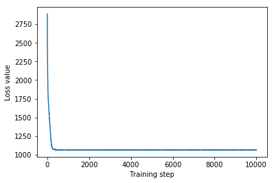
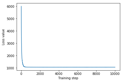
plt.plot(mvn_loss)
plt.xlabel('Training step')
_ = plt.ylabel('Loss value')
Multivariate Normal surrogate posterior ELBO: -1065.705322265625
از آنجایی که جایگزین آموزشدیده یک توزیع TFP است، میتوانیم نمونههایی از آن بگیریم و آنها را پردازش کنیم تا فواصل معتبر پسینی برای پارامترها تولید کنیم.
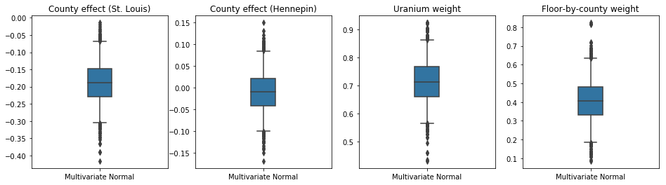
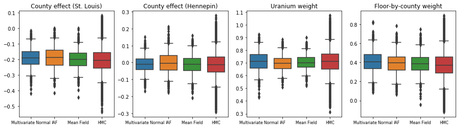
جعبه و سبیل توطئه زیر نشان می دهد 50٪ و 95٪ بازه مورد قبول برای اثر شهرستان از دو بزرگترین شهرستان و وزن های رگرسیون در اندازه گیری اورانیوم خاک و متوسط طبقه توسط استان. فواصل معتبر پسین برای اثرات شهرستان نشان می دهد که مکان در شهرستان سنت لوئیس با سطوح پایین تر رادون همراه است، پس از محاسبه سایر متغیرها، و اینکه اثر مکان در شهرستان هنپین نزدیک به خنثی است.
فواصل معتبر پسین روی وزنهای رگرسیون نشان میدهد که سطوح بالاتر اورانیوم خاک با سطوح بالاتر رادون مرتبط است و شهرستانهایی که اندازهگیریها در طبقات بالاتر انجام شده است (احتمالاً به دلیل نداشتن زیرزمین خانه) سطح بالاتری از رادون دارند. که می تواند به ویژگی های خاک و تأثیر آنها بر نوع سازه های ساخته شده مربوط باشد.
ضریب (قطعی) طبقه منفی است، که نشان می دهد طبقات پایین تر، همانطور که انتظار می رود، سطوح رادون بالاتری دارند.
st_louis_co = 69  # Index of St. Louis, the county with the most observations.
hennepin_co = 25  # Index of Hennepin, with the second-most observations.

def pack_samples(samples):
  return {'County effect (St. Louis)': samples.county_effect[..., st_louis_co],
          'County effect (Hennepin)': samples.county_effect[..., hennepin_co],
          'Uranium weight': samples.uranium_weight,
          'Floor-by-county weight': samples.county_floor_weight}

def plot_boxplot(posterior_samples):
  fig, axes = plt.subplots(1, 4, figsize=(16, 4))

  # Invert the results dict for easier plotting.
  k = list(posterior_samples.values())[0].keys()
  plot_results = {
      v: {p: posterior_samples[p][v] for p in posterior_samples} for v in k}
  for i, (var, var_results) in enumerate(plot_results.items()):
    sns.boxplot(data=list(var_results.values()), ax=axes[i],
                width=0.18*len(var_results), whis=(2.5, 97.5))
    # axes[i].boxplot(list(var_results.values()), whis=(2.5, 97.5))
    axes[i].title.set_text(var)
    fs = 10 if len(var_results) < 4 else 8
    axes[i].set_xticklabels(list(var_results.keys()), fontsize=fs)

results = {'Multivariate Normal': pack_samples(mvn_samples)}

print('Bias is: {:.2f}'.format(bias.numpy()))
print('Floor fixed effect is: {:.2f}'.format(floor_weight.numpy()))
plot_boxplot(results)
Bias is: 1.40
Floor fixed effect is: -0.72
جریان خودرگرسیون معکوس جانشین خلفی
جریانهای خودرگرسیون معکوس (IAF) جریانهای عادیسازی هستند که از شبکههای عصبی برای گرفتن وابستگیهای پیچیده و غیرخطی بین اجزای توزیع استفاده میکنند. در مرحله بعد، یک IAF جایگزین خلفی میسازیم تا ببینیم آیا این مدل با ظرفیت بالاتر و انعطافپذیرتر از نرمال چند متغیره محدود عملکرد بهتری دارد یا خیر.
# Build a standard Normal with a vector `event_shape`, with length equal to the
# total number of degrees of freedom in the posterior.
base_distribution = tfd.Sample(
    tfd.Normal(0., 1.), sample_shape=[tf.reduce_sum(flat_event_size)])

# Apply an IAF to the base distribution.
num_iafs = 2
iaf_bijectors = [
    tfb.Invert(tfb.MaskedAutoregressiveFlow(
        shift_and_log_scale_fn=tfb.AutoregressiveNetwork(
            params=2, hidden_units=[256, 256], activation='relu')))
    for _ in range(num_iafs)
]

# Split the base distribution's `event_shape` into components that are equal
# in size to the prior's components.
split = tfb.Split(flat_event_size)

# Chain these bijectors and apply them to the standard Normal base distribution
# to build the surrogate posterior. `event_space_bijector`,
# `unflatten_bijector`, and `reshape_bijector` are the same as in the
# multivariate Normal surrogate posterior.
iaf_surrogate_posterior = tfd.TransformedDistribution(
    base_distribution,
    bijector=tfb.Chain([
         event_space_bijector,  # constrain the surrogate to the support of the prior
         unflatten_bijector,  # pack the reshaped components into the `event_shape` structure of the prior
         reshape_bijector,  # reshape the vector-valued components to match the shapes of the prior components
         split] +  # Split the samples into components of the same size as the prior components
         iaf_bijectors  # Apply a flow model to the Tensor-valued standard Normal distribution
         ))
IAF جانشین خلفی را آموزش دهید.
optimizer=tf.optimizers.Adam(learning_rate=1e-2)
iaf_loss = tfp.vi.fit_surrogate_posterior(
target_model.unnormalized_log_prob,
iaf_surrogate_posterior,
optimizer=optimizer,
num_steps=10**4,
sample_size=4,
jit_compile=True)
iaf_samples = iaf_surrogate_posterior.sample(1000)
iaf_final_elbo = tf.reduce_mean(
target_model.unnormalized_log_prob(*iaf_samples)
- iaf_surrogate_posterior.log_prob(iaf_samples))
print('IAF surrogate posterior ELBO: {}'.format(iaf_final_elbo))
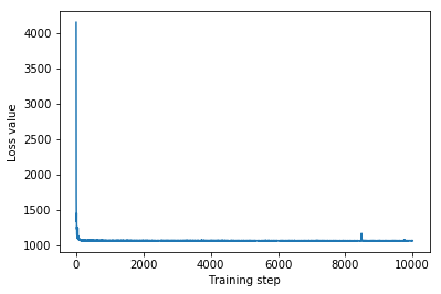
plt.plot(iaf_loss)
plt.xlabel('Training step')
_ = plt.ylabel('Loss value')
IAF surrogate posterior ELBO: -1065.3663330078125
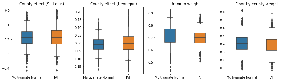
فواصل معتبر برای IAF جانشین خلفی شبیه به فواصل نرمال چند متغیره محدود به نظر می رسد.
results['IAF'] = pack_samples(iaf_samples)
plot_boxplot(results)
خط پایه: خلفی جایگزین میدان متوسط
غالباً فرض میشود که پستهای جانشین VI، توزیعهای نرمال میدان متوسط (مستقل)، با میانگینها و واریانسهای قابل آموزش هستند که به حمایت از قبلی با یک تبدیل دوطرفه محدود میشوند. ما با استفاده از فرمول کلی یکسانی به عنوان چند متغیره جایگزین خلفی عادی، علاوه بر دو جانشین خلفی گویاتر، یک جانشین با میدان متوسط را تعریف می کنیم.
# A block-diagonal linear operator, in which each block is a diagonal operator,
# transforms the standard Normal base distribution to produce a mean-field
# surrogate posterior.
operators = (tf.linalg.LinearOperatorDiag,
             tf.linalg.LinearOperatorDiag,
             tf.linalg.LinearOperatorDiag)
block_diag_linop = (
    tfp.experimental.vi.util.build_trainable_linear_operator_block(
        operators, flat_event_size))
mean_field_scale = tfb.ScaleMatvecLinearOperatorBlock(block_diag_linop)

mean_field_loc = tfb.JointMap(
    tf.nest.map_structure(
        lambda s: tfb.Shift(
            tf.Variable(tf.random.uniform(
                (s,), minval=-2., maxval=2., dtype=tf.float32))),
        flat_event_size))

mean_field_surrogate_posterior = tfd.TransformedDistribution(
    base_standard_dist,
    bijector = tfb.Chain(  # Note that the chained bijectors are applied in reverse order
        [
         event_space_bijector,  # constrain the surrogate to the support of the prior
         unflatten_bijector,  # pack the reshaped components into the `event_shape` structure of the posterior
         reshape_bijector, # reshape the vector-valued components to match the shapes of the posterior components
         mean_field_loc,   # allow for nonzero mean
         mean_field_scale  # apply the block matrix transformation to the standard Normal distribution
         ]))

optimizer=tf.optimizers.Adam(learning_rate=1e-2)
mean_field_loss = tfp.vi.fit_surrogate_posterior(
    target_model.unnormalized_log_prob,
    mean_field_surrogate_posterior,
    optimizer=optimizer,
    num_steps=10**4,
    sample_size=16,
    jit_compile=True)

mean_field_samples = mean_field_surrogate_posterior.sample(1000)
mean_field_final_elbo = tf.reduce_mean(
    target_model.unnormalized_log_prob(*mean_field_samples)
    - mean_field_surrogate_posterior.log_prob(mean_field_samples))
print('Mean-field surrogate posterior ELBO: {}'.format(mean_field_final_elbo))

plt.plot(mean_field_loss)
plt.xlabel('Training step')
_ = plt.ylabel('Loss value')
Mean-field surrogate posterior ELBO: -1065.7652587890625
در این مورد، میانگین میدان خلفی خلفی نتایج مشابهی با خلفی های جایگزین گویاتر می دهد، که نشان می دهد این مدل ساده تر ممکن است برای کار استنتاج کافی باشد.
results['Mean Field'] = pack_samples(mean_field_samples)
plot_boxplot(results)
حقیقت اصلی: همیلتونی مونت کارلو (HMC)
ما از HMC برای تولید نمونههای «حقیقت زمینی» از خلفی واقعی، برای مقایسه با نتایج جانشینهای خلفی استفاده میکنیم.
num_chains = 8
num_leapfrog_steps = 3
step_size = 0.4
num_steps=20000

flat_event_shape = tf.nest.flatten(target_model.event_shape)
enum_components = list(range(len(flat_event_shape)))
bijector = tfb.Restructure(
    enum_components,
    tf.nest.pack_sequence_as(target_model.event_shape, enum_components))(
        target_model.experimental_default_event_space_bijector())

current_state = bijector(
    tf.nest.map_structure(
        lambda e: tf.zeros([num_chains] + list(e), dtype=tf.float32),
    target_model.event_shape))

hmc = tfp.mcmc.HamiltonianMonteCarlo(
    target_log_prob_fn=target_model.unnormalized_log_prob,
    num_leapfrog_steps=num_leapfrog_steps,
    step_size=[tf.fill(s.shape, step_size) for s in current_state])

hmc = tfp.mcmc.TransformedTransitionKernel(
    hmc, bijector)
hmc = tfp.mcmc.DualAveragingStepSizeAdaptation(
    hmc,
    num_adaptation_steps=int(num_steps // 2 * 0.8),
    target_accept_prob=0.9)

chain, is_accepted = tf.function(
    lambda current_state: tfp.mcmc.sample_chain(
        current_state=current_state,
        kernel=hmc,
        num_results=num_steps // 2,
        num_burnin_steps=num_steps // 2,
        trace_fn=lambda _, pkr:
        (pkr.inner_results.inner_results.is_accepted),
        ),
    autograph=False,
    jit_compile=True)(current_state)

accept_rate = tf.reduce_mean(tf.cast(is_accepted, tf.float32))
ess = tf.nest.map_structure(
    lambda c: tfp.mcmc.effective_sample_size(
        c,
        cross_chain_dims=1,
        filter_beyond_positive_pairs=True),
    chain)

r_hat = tf.nest.map_structure(tfp.mcmc.potential_scale_reduction, chain)
hmc_samples = pack_samples(
    tf.nest.pack_sequence_as(target_model.event_shape, chain))
print('Acceptance rate is {}'.format(accept_rate))
Acceptance rate is 0.9008625149726868
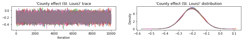
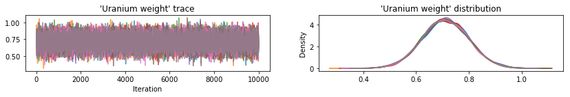
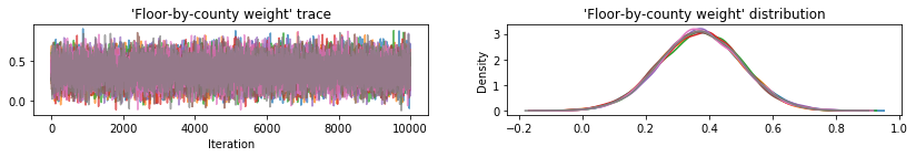
ردپای نمونه را برای بررسی سلامت عقل نتایج HMC ترسیم کنید.
def plot_traces(var_name, samples):
  fig, axes = plt.subplots(1, 2, figsize=(14, 1.5), sharex='col', sharey='col')
  for chain in range(num_chains):
    s = samples.numpy()[:, chain]
    axes[0].plot(s, alpha=0.7)
    sns.kdeplot(s, ax=axes[1], shade=False)
    axes[0].title.set_text("'{}' trace".format(var_name))
    axes[1].title.set_text("'{}' distribution".format(var_name))
    axes[0].set_xlabel('Iteration')

warnings.filterwarnings('ignore')
for var, var_samples in hmc_samples.items():
  plot_traces(var, var_samples)
هر سه جانشین خلفی فواصل معتبری را تولید کردند که از نظر بصری شبیه نمونههای HMC هستند، اگرچه گاهی اوقات به دلیل اثر از دست دادن ELBO کمتر پراکنده میشوند، همانطور که در VI رایج است.
results['HMC'] = hmc_samples
plot_boxplot(results)
نتایج اضافی
توابع رسم
plt.rcParams.update({'axes.titlesize': 'medium', 'xtick.labelsize': 'medium'})
def plot_loss_and_elbo():
  fig, axes = plt.subplots(1, 2, figsize=(12, 4))

  axes[0].scatter([0, 1, 2],
                  [mvn_final_elbo.numpy(),
                  iaf_final_elbo.numpy(),
                  mean_field_final_elbo.numpy()])
  axes[0].set_xticks(ticks=[0, 1, 2])
  axes[0].set_xticklabels(labels=[
    'Multivariate Normal', 'IAF', 'Mean Field'])
  axes[0].title.set_text('Evidence Lower Bound (ELBO)')

  axes[1].plot(mvn_loss, label='Multivariate Normal')
  axes[1].plot(iaf_loss, label='IAF')
  axes[1].plot(mean_field_loss, label='Mean Field')
  axes[1].set_ylim([1000, 4000])
  axes[1].set_xlabel('Training step')
  axes[1].set_ylabel('Loss (negative ELBO)')
  axes[1].title.set_text('Loss')
  plt.legend()
  plt.show()

plt.rcParams.update({'axes.titlesize': 'medium', 'xtick.labelsize': 'small'})
def plot_kdes(num_chains=8):
  fig, axes = plt.subplots(2, 2, figsize=(12, 8))
  k = list(results.values())[0].keys()
  plot_results = {
      v: {p: results[p][v] for p in results} for v in k}
  for i, (var, var_results) in enumerate(plot_results.items()):
    ax = axes[i % 2, i // 2]
    for posterior, posterior_results in var_results.items():
      if posterior == 'HMC':
        label = posterior
        for chain in range(num_chains):
          sns.kdeplot(
              posterior_results[:, chain],
              ax=ax, shade=False, color='k', linestyle=':', label=label)
          label=None
      else:
        sns.kdeplot(
            posterior_results, ax=ax, shade=False, label=posterior)
        ax.title.set_text('{}'.format(var))
    ax.legend()
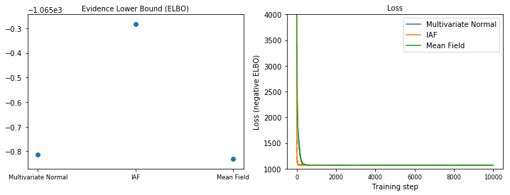
کران پایین شواهد (ELBO)
IAF، تا حد زیادی بزرگترین و منعطف ترین جانشین خلفی، به بالاترین حد پایین شواهد (ELBO) همگرا می شود.
plot_loss_and_elbo()
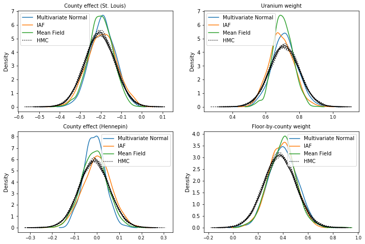
نمونه های خلفی
نمونهها از هر جانشین خلفی، در مقایسه با نمونههای حقیقت زمینی HMC (تجسم متفاوتی از نمونههای نشان داده شده در نمودارهای جعبه).
plot_kdes()
نتیجه
در این Colab، ما با استفاده از توزیعهای مشترک و بیژکتورهای چند قسمتی، قسمتهای خلفی جانشین VI را ساختیم و آنها را برای تخمین فواصل معتبر برای وزنها در یک مدل رگرسیون بر روی مجموعه داده رادون قرار دادیم. برای این مدل ساده، خلفی های جانشین رساتر به طور مشابه به خلفی جانشین با میدان متوسط عمل می کنند. ابزارهایی که نشان دادیم، با این حال، میتوانند برای ساخت طیف وسیعی از جانشینهای خلفی انعطافپذیر مناسب برای مدلهای پیچیدهتر استفاده شوند.