
| | |  GitHub पर स्रोत देखें GitHub पर स्रोत देखें | |
यह ट्यूटोरियल प्रदर्शित करता है कि कैसे WAV प्रारूप में ऑडियो फाइलों को प्रीप्रोसेस किया जाए और दस अलग-अलग शब्दों को पहचानने के लिए एक बुनियादी स्वचालित वाक् पहचान (ASR) मॉडल का निर्माण और प्रशिक्षण दिया जाए। आप स्पीच कमांड डेटासेट ( वार्डन, 2018 ) के एक हिस्से का उपयोग करेंगे, जिसमें कमांड के छोटे (एक सेकंड या उससे कम) ऑडियो क्लिप होते हैं, जैसे "डाउन", "गो", "लेफ्ट", "नो", " राइट", "स्टॉप", "अप" और "हां"।
वास्तविक-विश्व भाषण और ऑडियो पहचान प्रणाली जटिल हैं। लेकिन, MNIST डेटासेट के साथ छवि वर्गीकरण की तरह, यह ट्यूटोरियल आपको शामिल तकनीकों की एक बुनियादी समझ प्रदान करेगा।
सेट अप
आवश्यक मॉड्यूल और निर्भरता आयात करें। ध्यान दें कि आप इस ट्यूटोरियल में विज़ुअलाइज़ेशन के लिए सीबॉर्न का उपयोग करेंगे।
import os
import pathlib

import matplotlib.pyplot as plt
import numpy as np
import seaborn as sns
import tensorflow as tf

from tensorflow.keras import layers
from tensorflow.keras import models
from IPython import display

# Set the seed value for experiment reproducibility.
seed = 42
tf.random.set_seed(seed)
np.random.seed(seed)
मिनी स्पीच कमांड डेटासेट आयात करें
डेटा लोड करने में समय बचाने के लिए, आप स्पीच कमांड डेटासेट के एक छोटे संस्करण के साथ काम करेंगे। मूल डेटासेट में WAV (वेवफॉर्म) ऑडियो फ़ाइल स्वरूप में 105,000 से अधिक ऑडियो फ़ाइलें होती हैं, जिनमें 35 अलग-अलग शब्द कहने वाले लोग होते हैं। यह डेटा Google द्वारा एकत्र किया गया था और CC BY लाइसेंस के तहत जारी किया गया था।
tf.keras.utils.get_file के साथ छोटे स्पीच कमांड डेटासेट वाली mini_speech_commands.zip फ़ाइल डाउनलोड करें और निकालें:
DATASET_PATH = 'data/mini_speech_commands'

data_dir = pathlib.Path(DATASET_PATH)
if not data_dir.exists():
  tf.keras.utils.get_file(
      'mini_speech_commands.zip',
      origin="http://storage.googleapis.com/download.tensorflow.org/data/mini_speech_commands.zip",
      extract=True,
      cache_dir='.', cache_subdir='data')
Downloading data from http://storage.googleapis.com/download.tensorflow.org/data/mini_speech_commands.zip
182083584/182082353 [==============================] - 1s 0us/step
182091776/182082353 [==============================] - 1s 0us/step
डेटासेट की ऑडियो क्लिप प्रत्येक स्पीच कमांड के अनुरूप आठ फ़ोल्डरों में संग्रहीत की जाती हैं: no , yes , down , go , left , up , right , और stop :
commands = np.array(tf.io.gfile.listdir(str(data_dir)))
commands = commands[commands != 'README.md']
print('Commands:', commands)
Commands: ['stop' 'left' 'no' 'go' 'yes' 'down' 'right' 'up']
filenames नामक सूची में ऑडियो क्लिप निकालें, और इसे शफ़ल करें:
filenames = tf.io.gfile.glob(str(data_dir) + '/*/*')
filenames = tf.random.shuffle(filenames)
num_samples = len(filenames)
print('Number of total examples:', num_samples)
print('Number of examples per label:',
      len(tf.io.gfile.listdir(str(data_dir/commands[0]))))
print('Example file tensor:', filenames[0])
Number of total examples: 8000
Number of examples per label: 1000
Example file tensor: tf.Tensor(b'data/mini_speech_commands/yes/db72a474_nohash_0.wav', shape=(), dtype=string)
filenames को क्रमशः 80:10:10 अनुपात का उपयोग करके प्रशिक्षण, सत्यापन और परीक्षण सेट में विभाजित करें:
train_files = filenames[:6400]
val_files = filenames[6400: 6400 + 800]
test_files = filenames[-800:]

print('Training set size', len(train_files))
print('Validation set size', len(val_files))
print('Test set size', len(test_files))
Training set size 6400
Validation set size 800
Test set size 800
ऑडियो फ़ाइलें और उनके लेबल पढ़ें
इस खंड में आप डेटासेट को प्रीप्रोसेस करेंगे, वेवफॉर्म और संबंधित लेबल के लिए डिकोडेड टेंसर बनाएंगे। ध्यान दें कि:
- प्रत्येक WAV फ़ाइल में प्रति सेकंड नमूनों की एक निर्धारित संख्या के साथ समय-श्रृंखला डेटा होता है।
- प्रत्येक नमूना उस विशिष्ट समय पर ऑडियो सिग्नल के आयाम का प्रतिनिधित्व करता है।
- 16-बिट सिस्टम में, मिनी स्पीच कमांड डेटासेट में WAV फ़ाइलों की तरह, आयाम मान -32,768 से 32,767 तक होते हैं।
- इस डेटासेट के लिए नमूना दर 16kHz है।
tf.audio.decode_wav द्वारा लौटाए गए टेंसर का आकार [samples, channels] है, जहां channels मोनो के लिए 1 या स्टीरियो के लिए 2 है। मिनी स्पीच कमांड डेटासेट में केवल मोनो रिकॉर्डिंग होती है।
test_file = tf.io.read_file(DATASET_PATH+'/down/0a9f9af7_nohash_0.wav')
test_audio, _ = tf.audio.decode_wav(contents=test_file)
test_audio.shape
TensorShape([13654, 1])
अब, एक फ़ंक्शन को परिभाषित करते हैं जो डेटासेट की कच्ची WAV ऑडियो फ़ाइलों को ऑडियो टेंसर में प्रीप्रोसेस करता है:
def decode_audio(audio_binary):
  # Decode WAV-encoded audio files to `float32` tensors, normalized
  # to the [-1.0, 1.0] range. Return `float32` audio and a sample rate.
  audio, _ = tf.audio.decode_wav(contents=audio_binary)
  # Since all the data is single channel (mono), drop the `channels`
  # axis from the array.
  return tf.squeeze(audio, axis=-1)
प्रत्येक फ़ाइल के लिए मूल निर्देशिकाओं का उपयोग करके लेबल बनाने वाले फ़ंक्शन को परिभाषित करें:
- फ़ाइल पथों को
tf.RaggedTensors में विभाजित करें (रैग्ड आयामों वाले टेंसर-स्लाइस के साथ जिनकी लंबाई अलग-अलग हो सकती है)।
def get_label(file_path):
  parts = tf.strings.split(
      input=file_path,
      sep=os.path.sep)
  # Note: You'll use indexing here instead of tuple unpacking to enable this
  # to work in a TensorFlow graph.
  return parts[-2]
एक अन्य सहायक फ़ंक्शन को परिभाषित get_waveform_and_label इसे एक साथ रखता है:
- इनपुट WAV ऑडियो फ़ाइल नाम है।
- आउटपुट एक टपल है जिसमें पर्यवेक्षित सीखने के लिए तैयार ऑडियो और लेबल टेंसर होते हैं।
def get_waveform_and_label(file_path):
  label = get_label(file_path)
  audio_binary = tf.io.read_file(file_path)
  waveform = decode_audio(audio_binary)
  return waveform, label
ऑडियो-लेबल जोड़े निकालने के लिए प्रशिक्षण सेट बनाएँ:
- पहले परिभाषित
get_waveform_and_labelका उपयोग करकेDataset.from_tensor_slicesऔरDataset.mapके साथ एकtf.data.Datasetबनाएं।
आप बाद में इसी तरह की प्रक्रिया का उपयोग करके सत्यापन और परीक्षण सेट तैयार करेंगे।
AUTOTUNE = tf.data.AUTOTUNE

files_ds = tf.data.Dataset.from_tensor_slices(train_files)

waveform_ds = files_ds.map(
    map_func=get_waveform_and_label,
    num_parallel_calls=AUTOTUNE)
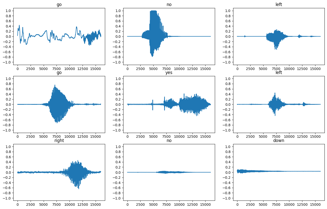
आइए कुछ ऑडियो तरंगों को प्लॉट करें:
rows = 3
cols = 3
n = rows * cols
fig, axes = plt.subplots(rows, cols, figsize=(10, 12))

for i, (audio, label) in enumerate(waveform_ds.take(n)):
  r = i // cols
  c = i % cols
  ax = axes[r][c]
  ax.plot(audio.numpy())
  ax.set_yticks(np.arange(-1.2, 1.2, 0.2))
  label = label.numpy().decode('utf-8')
  ax.set_title(label)

plt.show()
तरंगों को स्पेक्ट्रोग्राम में बदलें
डेटासेट में तरंगों को समय क्षेत्र में दर्शाया जाता है। इसके बाद, आप तरंगों को समय-क्षेत्र संकेतों से समय-आवृत्ति-डोमेन संकेतों में परिवर्तित करेंगे, तरंगों को स्पेक्ट्रोग्राम के रूप में परिवर्तित करने के लिए शॉर्ट-टाइम फूरियर ट्रांसफॉर्म (एसटीएफटी) की गणना करके, जो समय के साथ आवृत्ति परिवर्तन दिखाते हैं और हो सकते हैं 2डी छवियों के रूप में प्रतिनिधित्व किया। आप मॉडल को प्रशिक्षित करने के लिए स्पेक्ट्रोग्राम छवियों को अपने तंत्रिका नेटवर्क में फीड करेंगे।
एक फूरियर ट्रांसफॉर्म ( tf.signal.fft ) एक सिग्नल को उसके घटक आवृत्तियों में परिवर्तित करता है, लेकिन सभी समय की जानकारी खो देता है। इसकी तुलना में, STFT ( tf.signal.stft ) सिग्नल को समय की खिड़कियों में विभाजित करता है और प्रत्येक विंडो पर एक फूरियर ट्रांसफॉर्म चलाता है, कुछ समय की जानकारी को संरक्षित करता है, और एक 2D टेंसर लौटाता है जिस पर आप मानक कनवल्शन चला सकते हैं।
तरंगों को स्पेक्ट्रोग्राम में बदलने के लिए एक उपयोगिता फ़ंक्शन बनाएं:
- तरंगों को समान लंबाई का होना चाहिए, ताकि जब आप उन्हें स्पेक्ट्रोग्राम में परिवर्तित करें, तो परिणाम समान आयाम हों। यह केवल एक सेकंड से छोटे ऑडियो क्लिप को शून्य-पैडिंग करके किया जा सकता है (
tf.zerosका उपयोग करके)। -
tf.signal.stftको कॉल करते समय,frame_lengthऔरframe_stepपैरामीटर चुनें जैसे कि उत्पन्न स्पेक्ट्रोग्राम "इमेज" लगभग चौकोर हो। एसटीएफटी मापदंडों की पसंद के बारे में अधिक जानकारी के लिए, ऑडियो सिग्नल प्रोसेसिंग और एसटीएफटी पर इस कौरसेरा वीडियो को देखें। - एसटीएफटी परिमाण और चरण का प्रतिनिधित्व करने वाली जटिल संख्याओं की एक सरणी तैयार करता है। हालाँकि, इस ट्यूटोरियल में आप केवल उस परिमाण का उपयोग करेंगे, जिसे आप
tf.signal.stftके आउटपुट परtf.absलागू करके प्राप्त कर सकते हैं।
def get_spectrogram(waveform):
  # Zero-padding for an audio waveform with less than 16,000 samples.
  input_len = 16000
  waveform = waveform[:input_len]
  zero_padding = tf.zeros(
      [16000] - tf.shape(waveform),
      dtype=tf.float32)
  # Cast the waveform tensors' dtype to float32.
  waveform = tf.cast(waveform, dtype=tf.float32)
  # Concatenate the waveform with `zero_padding`, which ensures all audio
  # clips are of the same length.
  equal_length = tf.concat([waveform, zero_padding], 0)
  # Convert the waveform to a spectrogram via a STFT.
  spectrogram = tf.signal.stft(
      equal_length, frame_length=255, frame_step=128)
  # Obtain the magnitude of the STFT.
  spectrogram = tf.abs(spectrogram)
  # Add a `channels` dimension, so that the spectrogram can be used
  # as image-like input data with convolution layers (which expect
  # shape (`batch_size`, `height`, `width`, `channels`).
  spectrogram = spectrogram[..., tf.newaxis]
  return spectrogram
इसके बाद, डेटा की खोज शुरू करें। एक उदाहरण के टेंसराइज्ड वेवफॉर्म और संबंधित स्पेक्ट्रोग्राम के आकार को प्रिंट करें, और मूल ऑडियो चलाएं:
for waveform, label in waveform_ds.take(1):
  label = label.numpy().decode('utf-8')
  spectrogram = get_spectrogram(waveform)

print('Label:', label)
print('Waveform shape:', waveform.shape)
print('Spectrogram shape:', spectrogram.shape)
print('Audio playback')
display.display(display.Audio(waveform, rate=16000))
Label: yes
Waveform shape: (16000,)
Spectrogram shape: (124, 129, 1)
Audio playback
अब, एक स्पेक्ट्रोग्राम प्रदर्शित करने के लिए एक फ़ंक्शन को परिभाषित करें:
def plot_spectrogram(spectrogram, ax):
  if len(spectrogram.shape) > 2:
    assert len(spectrogram.shape) == 3
    spectrogram = np.squeeze(spectrogram, axis=-1)
  # Convert the frequencies to log scale and transpose, so that the time is
  # represented on the x-axis (columns).
  # Add an epsilon to avoid taking a log of zero.
  log_spec = np.log(spectrogram.T + np.finfo(float).eps)
  height = log_spec.shape[0]
  width = log_spec.shape[1]
  X = np.linspace(0, np.size(spectrogram), num=width, dtype=int)
  Y = range(height)
  ax.pcolormesh(X, Y, log_spec)
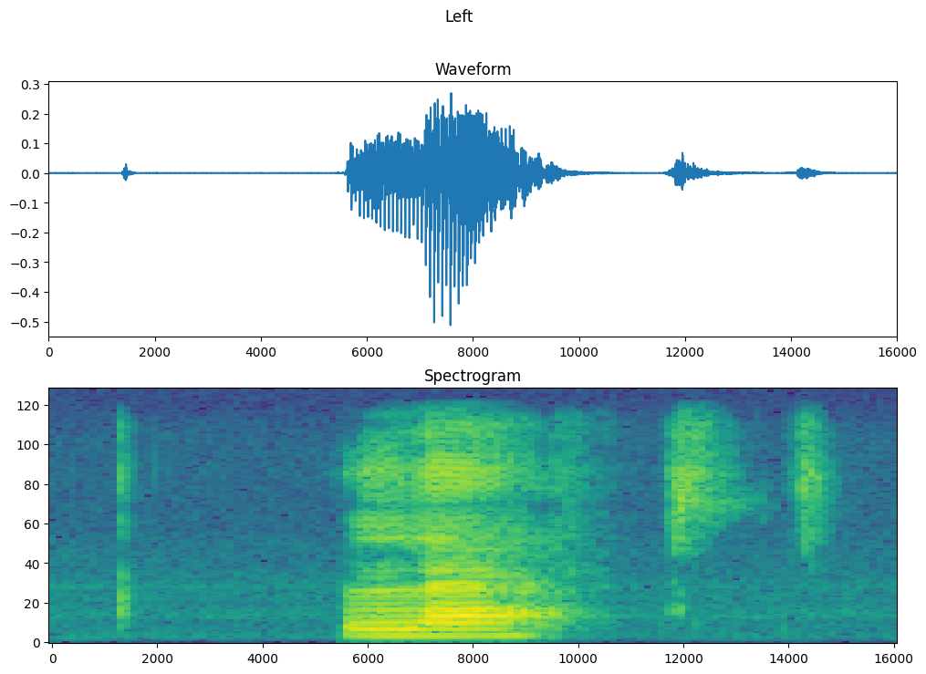
समय के साथ उदाहरण के तरंग और संबंधित स्पेक्ट्रोग्राम (समय के साथ आवृत्तियों) को प्लॉट करें:
fig, axes = plt.subplots(2, figsize=(12, 8))
timescale = np.arange(waveform.shape[0])
axes[0].plot(timescale, waveform.numpy())
axes[0].set_title('Waveform')
axes[0].set_xlim([0, 16000])

plot_spectrogram(spectrogram.numpy(), axes[1])
axes[1].set_title('Spectrogram')
plt.show()
अब, एक फ़ंक्शन को परिभाषित करें जो तरंग डेटासेट को स्पेक्ट्रोग्राम और उनके संबंधित लेबल को पूर्णांक आईडी के रूप में बदल देता है:
def get_spectrogram_and_label_id(audio, label):
  spectrogram = get_spectrogram(audio)
  label_id = tf.argmax(label == commands)
  return spectrogram, label_id
get_spectrogram_and_label_id के साथ डेटासेट के तत्वों में Dataset.map करें:
spectrogram_ds = waveform_ds.map(
  map_func=get_spectrogram_and_label_id,
  num_parallel_calls=AUTOTUNE)
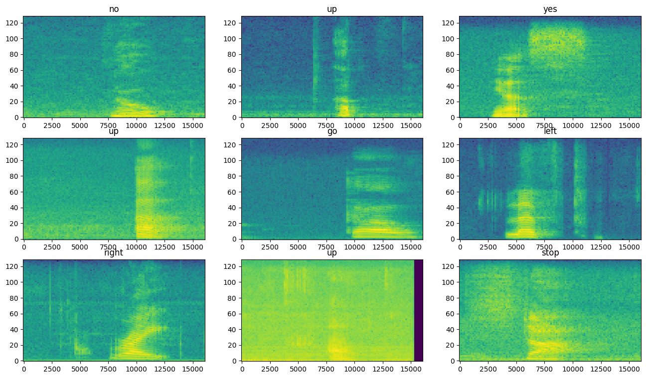
डेटासेट के विभिन्न उदाहरणों के लिए स्पेक्ट्रोग्राम की जांच करें:
rows = 3
cols = 3
n = rows*cols
fig, axes = plt.subplots(rows, cols, figsize=(10, 10))

for i, (spectrogram, label_id) in enumerate(spectrogram_ds.take(n)):
  r = i // cols
  c = i % cols
  ax = axes[r][c]
  plot_spectrogram(spectrogram.numpy(), ax)
  ax.set_title(commands[label_id.numpy()])
  ax.axis('off')

plt.show()
मॉडल बनाएं और प्रशिक्षित करें
सत्यापन और परीक्षण सेट पर प्रशिक्षण सेट प्रीप्रोसेसिंग दोहराएं:
def preprocess_dataset(files):
  files_ds = tf.data.Dataset.from_tensor_slices(files)
  output_ds = files_ds.map(
      map_func=get_waveform_and_label,
      num_parallel_calls=AUTOTUNE)
  output_ds = output_ds.map(
      map_func=get_spectrogram_and_label_id,
      num_parallel_calls=AUTOTUNE)
  return output_ds
train_ds = spectrogram_ds
val_ds = preprocess_dataset(val_files)
test_ds = preprocess_dataset(test_files)
मॉडल प्रशिक्षण के लिए बैच प्रशिक्षण और सत्यापन सेट:
batch_size = 64
train_ds = train_ds.batch(batch_size)
val_ds = val_ds.batch(batch_size)
मॉडल को प्रशिक्षित करते समय पढ़ने की विलंबता को कम करने के लिए Dataset.cache और Dataset.prefetch संचालन जोड़ें:
train_ds = train_ds.cache().prefetch(AUTOTUNE)
val_ds = val_ds.cache().prefetch(AUTOTUNE)
मॉडल के लिए, आप एक साधारण कनवल्शनल न्यूरल नेटवर्क (CNN) का उपयोग करेंगे, क्योंकि आपने ऑडियो फ़ाइलों को स्पेक्ट्रोग्राम छवियों में बदल दिया है।
आपका tf.keras.Sequential मॉडल निम्नलिखित केरस प्रीप्रोसेसिंग परतों का उपयोग करेगा:
-
tf.keras.layers.Resizing: मॉडल को तेजी से प्रशिक्षित करने के लिए इनपुट को कम करने के लिए। -
tf.keras.layers.Normalization: छवि में प्रत्येक पिक्सेल को उसके माध्य और मानक विचलन के आधार पर सामान्य करने के लिए।
Normalization परत के लिए, समग्र आँकड़ों (अर्थात, माध्य और मानक विचलन) की गणना करने के लिए पहले इसकी adapt विधि को प्रशिक्षण डेटा पर कॉल करने की आवश्यकता होगी।
for spectrogram, _ in spectrogram_ds.take(1):
  input_shape = spectrogram.shape
print('Input shape:', input_shape)
num_labels = len(commands)

# Instantiate the `tf.keras.layers.Normalization` layer.
norm_layer = layers.Normalization()
# Fit the state of the layer to the spectrograms
# with `Normalization.adapt`.
norm_layer.adapt(data=spectrogram_ds.map(map_func=lambda spec, label: spec))

model = models.Sequential([
    layers.Input(shape=input_shape),
    # Downsample the input.
    layers.Resizing(32, 32),
    # Normalize.
    norm_layer,
    layers.Conv2D(32, 3, activation='relu'),
    layers.Conv2D(64, 3, activation='relu'),
    layers.MaxPooling2D(),
    layers.Dropout(0.25),
    layers.Flatten(),
    layers.Dense(128, activation='relu'),
    layers.Dropout(0.5),
    layers.Dense(num_labels),
])

model.summary()
Input shape: (124, 129, 1)
Model: "sequential"
_________________________________________________________________
 Layer (type)                Output Shape              Param #
=================================================================
 resizing (Resizing)         (None, 32, 32, 1)         0

 normalization (Normalizatio  (None, 32, 32, 1)        3
 n)

 conv2d (Conv2D)             (None, 30, 30, 32)        320

 conv2d_1 (Conv2D)           (None, 28, 28, 64)        18496

 max_pooling2d (MaxPooling2D  (None, 14, 14, 64)       0
 )

 dropout (Dropout)           (None, 14, 14, 64)        0

 flatten (Flatten)           (None, 12544)             0

 dense (Dense)               (None, 128)               1605760

 dropout_1 (Dropout)         (None, 128)               0

 dense_1 (Dense)             (None, 8)                 1032

=================================================================
Total params: 1,625,611
Trainable params: 1,625,608
Non-trainable params: 3
_________________________________________________________________
एडम ऑप्टिमाइज़र और क्रॉस-एन्ट्रापी लॉस के साथ केरस मॉडल को कॉन्फ़िगर करें:
model.compile(
    optimizer=tf.keras.optimizers.Adam(),
    loss=tf.keras.losses.SparseCategoricalCrossentropy(from_logits=True),
    metrics=['accuracy'],
)
प्रदर्शन उद्देश्यों के लिए 10 से अधिक युगों में मॉडल को प्रशिक्षित करें:
EPOCHS = 10
history = model.fit(
    train_ds,
    validation_data=val_ds,
    epochs=EPOCHS,
    callbacks=tf.keras.callbacks.EarlyStopping(verbose=1, patience=2),
)
Epoch 1/10
100/100 [==============================] - 6s 41ms/step - loss: 1.7503 - accuracy: 0.3630 - val_loss: 1.2850 - val_accuracy: 0.5763
Epoch 2/10
100/100 [==============================] - 0s 5ms/step - loss: 1.2101 - accuracy: 0.5698 - val_loss: 0.9314 - val_accuracy: 0.6913
Epoch 3/10
100/100 [==============================] - 0s 5ms/step - loss: 0.9336 - accuracy: 0.6703 - val_loss: 0.7529 - val_accuracy: 0.7325
Epoch 4/10
100/100 [==============================] - 0s 5ms/step - loss: 0.7503 - accuracy: 0.7397 - val_loss: 0.6721 - val_accuracy: 0.7713
Epoch 5/10
100/100 [==============================] - 0s 5ms/step - loss: 0.6367 - accuracy: 0.7741 - val_loss: 0.6061 - val_accuracy: 0.7975
Epoch 6/10
100/100 [==============================] - 0s 5ms/step - loss: 0.5650 - accuracy: 0.7987 - val_loss: 0.5489 - val_accuracy: 0.8125
Epoch 7/10
100/100 [==============================] - 0s 5ms/step - loss: 0.5099 - accuracy: 0.8183 - val_loss: 0.5344 - val_accuracy: 0.8238
Epoch 8/10
100/100 [==============================] - 0s 5ms/step - loss: 0.4560 - accuracy: 0.8392 - val_loss: 0.5194 - val_accuracy: 0.8288
Epoch 9/10
100/100 [==============================] - 0s 5ms/step - loss: 0.4101 - accuracy: 0.8547 - val_loss: 0.4809 - val_accuracy: 0.8388
Epoch 10/10
100/100 [==============================] - 0s 5ms/step - loss: 0.3905 - accuracy: 0.8589 - val_loss: 0.4973 - val_accuracy: 0.8363
प्लेसहोल्डर33
प्रशिक्षण के दौरान आपके मॉडल में कैसे सुधार हुआ है, यह जांचने के लिए प्रशिक्षण और सत्यापन हानि वक्रों की साजिश करें:
metrics = history.history
plt.plot(history.epoch, metrics['loss'], metrics['val_loss'])
plt.legend(['loss', 'val_loss'])
plt.show()

मॉडल के प्रदर्शन का मूल्यांकन करें
परीक्षण सेट पर मॉडल चलाएँ और मॉडल के प्रदर्शन की जाँच करें:
test_audio = []
test_labels = []

for audio, label in test_ds:
  test_audio.append(audio.numpy())
  test_labels.append(label.numpy())

test_audio = np.array(test_audio)
test_labels = np.array(test_labels)
y_pred = np.argmax(model.predict(test_audio), axis=1)
y_true = test_labels

test_acc = sum(y_pred == y_true) / len(y_true)
print(f'Test set accuracy: {test_acc:.0%}')
Test set accuracy: 85%
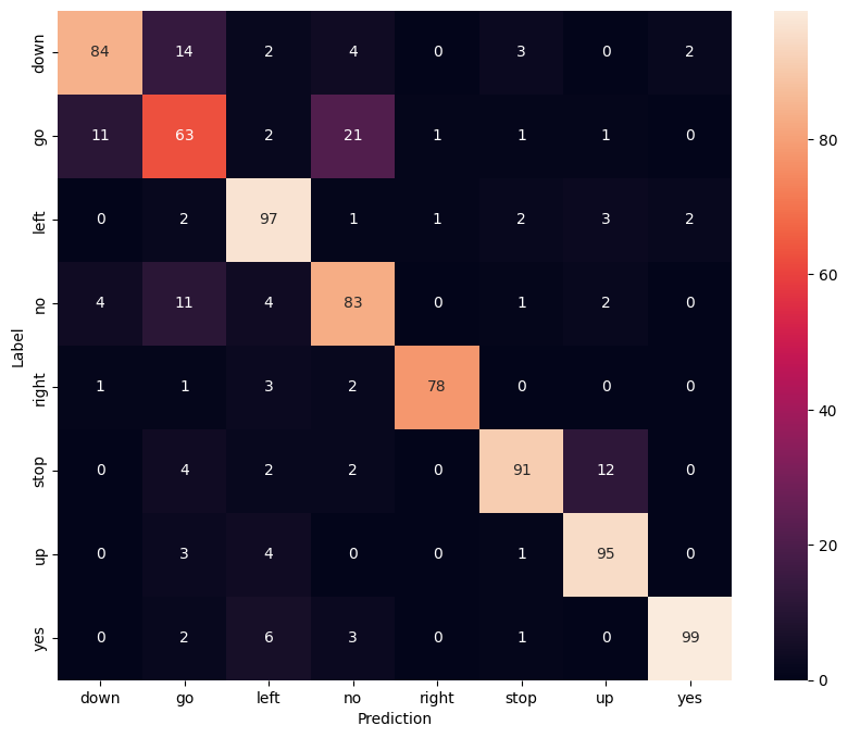
एक भ्रम मैट्रिक्स प्रदर्शित करें
परीक्षण सेट में प्रत्येक कमांड को वर्गीकृत करने के लिए मॉडल ने कितनी अच्छी तरह से जांच करने के लिए एक भ्रम मैट्रिक्स का उपयोग करें:
confusion_mtx = tf.math.confusion_matrix(y_true, y_pred)
plt.figure(figsize=(10, 8))
sns.heatmap(confusion_mtx,
            xticklabels=commands,
            yticklabels=commands,
            annot=True, fmt='g')
plt.xlabel('Prediction')
plt.ylabel('Label')
plt.show()
ऑडियो फ़ाइल पर अनुमान चलाएँ
अंत में, "नहीं" कहने वाले किसी व्यक्ति की इनपुट ऑडियो फ़ाइल का उपयोग करके मॉडल के पूर्वानुमान आउटपुट को सत्यापित करें। आपका मॉडल कितना अच्छा प्रदर्शन करता है?
sample_file = data_dir/'no/01bb6a2a_nohash_0.wav'

sample_ds = preprocess_dataset([str(sample_file)])

for spectrogram, label in sample_ds.batch(1):
  prediction = model(spectrogram)
  plt.bar(commands, tf.nn.softmax(prediction[0]))
  plt.title(f'Predictions for "{commands[label[0]]}"')
  plt.show()
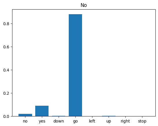
जैसा कि आउटपुट से पता चलता है, आपके मॉडल को ऑडियो कमांड को "नहीं" के रूप में पहचानना चाहिए था।
अगले कदम
इस ट्यूटोरियल ने प्रदर्शित किया कि TensorFlow और Python के साथ एक दृढ़ तंत्रिका नेटवर्क का उपयोग करके सरल ऑडियो वर्गीकरण/स्वचालित भाषण पहचान कैसे करें। अधिक जानने के लिए, निम्नलिखित संसाधनों पर विचार करें:
- YAMNet ट्यूटोरियल के साथ ध्वनि वर्गीकरण दिखाता है कि ऑडियो वर्गीकरण के लिए ट्रांसफर लर्निंग का उपयोग कैसे किया जाता है।
- कागल के TensorFlow वाक् पहचान चुनौती से नोटबुक।
- TensorFlow.js - ट्रांसफर लर्निंग कोडलैब का उपयोग करके ऑडियो पहचान सिखाती है कि ऑडियो वर्गीकरण के लिए अपना खुद का इंटरैक्टिव वेब ऐप कैसे बनाया जाए।
- संगीत सूचना पुनर्प्राप्ति के लिए गहन शिक्षण पर एक ट्यूटोरियल (चोई एट अल।, 2017) arXiv पर।
- TensorFlow में ऑडियो डेटा तैयार करने और आपके स्वयं के ऑडियो-आधारित प्रोजेक्ट में मदद करने के लिए वृद्धि के लिए अतिरिक्त समर्थन भी है।
- संगीत और ऑडियो विश्लेषण के लिए लिब्रोसा लाइब्रेरी—पायथन पैकेज का उपयोग करने पर विचार करें।