
| | |  ดูแหล่งที่มาบน GitHub ดูแหล่งที่มาบน GitHub | |
บทช่วยสอนนี้สาธิตวิธีประมวลผลไฟล์เสียงล่วงหน้าในรูปแบบ WAV และสร้างและฝึกโมเดล การรู้จำเสียงอัตโนมัติ (ASR) ขั้นพื้นฐานสำหรับการจำแนกคำสิบคำที่แตกต่างกัน คุณจะใช้ส่วนหนึ่งของ ชุดข้อมูล Speech Commands ( Warden, 2018 ) ซึ่งมีคลิปเสียงสั้นๆ (หนึ่งวินาทีหรือน้อยกว่า) ของคำสั่ง เช่น "ลง", "ไป", "ซ้าย", "ไม่", " ขวา", "หยุด", "ขึ้น" และ "ใช่"
ระบบ การรู้จำเสียงพูดและเสียงในโลกแห่งความเป็นจริงนั้นซับซ้อน แต่เช่นเดียว กับการจัดประเภทรูปภาพด้วยชุดข้อมูล MNIST บทช่วยสอนนี้ควรให้ความเข้าใจพื้นฐานเกี่ยวกับเทคนิคที่เกี่ยวข้องแก่คุณ
ติดตั้ง
นำเข้าโมดูลและการอ้างอิงที่จำเป็น โปรดทราบว่าคุณจะใช้ Seaborn สำหรับการสร้างภาพข้อมูลในบทช่วยสอนนี้
import os
import pathlib

import matplotlib.pyplot as plt
import numpy as np
import seaborn as sns
import tensorflow as tf

from tensorflow.keras import layers
from tensorflow.keras import models
from IPython import display

# Set the seed value for experiment reproducibility.
seed = 42
tf.random.set_seed(seed)
np.random.seed(seed)
นำเข้าชุดข้อมูลคำสั่งคำพูดขนาดเล็ก
เพื่อประหยัดเวลาในการโหลดข้อมูล คุณจะต้องทำงานกับชุดข้อมูลคำสั่งคำพูดเวอร์ชันที่เล็กกว่า ชุดข้อมูลดั้งเดิม ประกอบด้วยไฟล์เสียงมากกว่า 105,000 ไฟล์ใน รูปแบบไฟล์เสียง WAV (Waveform) ของผู้คนที่พูด 35 คำที่แตกต่างกัน ข้อมูลนี้รวบรวมโดย Google และเผยแพร่ภายใต้ใบอนุญาต CC BY
ดาวน์โหลดและแตกไฟล์ mini_speech_commands.zip ที่มีชุดข้อมูล Speech Commands ที่เล็กกว่าด้วย tf.keras.utils.get_file :
DATASET_PATH = 'data/mini_speech_commands'

data_dir = pathlib.Path(DATASET_PATH)
if not data_dir.exists():
  tf.keras.utils.get_file(
      'mini_speech_commands.zip',
      origin="http://storage.googleapis.com/download.tensorflow.org/data/mini_speech_commands.zip",
      extract=True,
      cache_dir='.', cache_subdir='data')
Downloading data from http://storage.googleapis.com/download.tensorflow.org/data/mini_speech_commands.zip
182083584/182082353 [==============================] - 1s 0us/step
182091776/182082353 [==============================] - 1s 0us/step
คลิปเสียงของชุดข้อมูลถูกจัดเก็บไว้ในโฟลเดอร์แปดโฟลเดอร์ที่สอดคล้องกับคำสั่งเสียงพูดแต่ละคำสั่ง: no , yes , down , go , left , up , right , and stop :
commands = np.array(tf.io.gfile.listdir(str(data_dir)))
commands = commands[commands != 'README.md']
print('Commands:', commands)
Commands: ['stop' 'left' 'no' 'go' 'yes' 'down' 'right' 'up']
แยกคลิปเสียงลงในรายการที่เรียกว่า filenames และสับเปลี่ยน:
filenames = tf.io.gfile.glob(str(data_dir) + '/*/*')
filenames = tf.random.shuffle(filenames)
num_samples = len(filenames)
print('Number of total examples:', num_samples)
print('Number of examples per label:',
      len(tf.io.gfile.listdir(str(data_dir/commands[0]))))
print('Example file tensor:', filenames[0])
Number of total examples: 8000
Number of examples per label: 1000
Example file tensor: tf.Tensor(b'data/mini_speech_commands/yes/db72a474_nohash_0.wav', shape=(), dtype=string)
แบ่ง filenames ออกเป็นชุดการฝึก การตรวจสอบ และการทดสอบโดยใช้อัตราส่วน 80:10:10 ตามลำดับ:
train_files = filenames[:6400]
val_files = filenames[6400: 6400 + 800]
test_files = filenames[-800:]

print('Training set size', len(train_files))
print('Validation set size', len(val_files))
print('Test set size', len(test_files))
Training set size 6400
Validation set size 800
Test set size 800
อ่านไฟล์เสียงและป้ายกำกับ
ในส่วนนี้ คุณจะประมวลผลชุดข้อมูลล่วงหน้า โดยสร้างเมตริกซ์ถอดรหัสสำหรับรูปคลื่นและป้ายกำกับที่เกี่ยวข้อง โปรดทราบว่า:
- ไฟล์ WAV แต่ละไฟล์มีข้อมูลอนุกรมเวลาพร้อมจำนวนชุดตัวอย่างต่อวินาที
- แต่ละตัวอย่างแสดงถึง แอมพลิจูด ของสัญญาณเสียง ณ เวลาที่กำหนด
- ในระบบ 16 บิต เช่น ไฟล์ WAV ในชุดข้อมูลคำสั่งเสียงพูดขนาดเล็ก ค่าแอมพลิจูดมีตั้งแต่ -32,768 ถึง 32,767
- อัตราสุ่ม สำหรับชุดข้อมูลนี้คือ 16kHz
รูปร่างของเทนเซอร์ที่ส่งคืนโดย tf.audio.decode_wav คือ [samples, channels] โดยที่ channels คือ 1 สำหรับโมโนหรือ 2 สำหรับสเตอริโอ ชุดข้อมูลคำสั่งเสียงพูดขนาดเล็กมีการบันทึกแบบโมโนเท่านั้น
test_file = tf.io.read_file(DATASET_PATH+'/down/0a9f9af7_nohash_0.wav')
test_audio, _ = tf.audio.decode_wav(contents=test_file)
test_audio.shape
TensorShape([13654, 1])
ตอนนี้ มากำหนดฟังก์ชั่นที่ประมวลผลไฟล์เสียง WAV แบบ raw ของชุดข้อมูลเป็นเทนเซอร์เสียง:
def decode_audio(audio_binary):
  # Decode WAV-encoded audio files to `float32` tensors, normalized
  # to the [-1.0, 1.0] range. Return `float32` audio and a sample rate.
  audio, _ = tf.audio.decode_wav(contents=audio_binary)
  # Since all the data is single channel (mono), drop the `channels`
  # axis from the array.
  return tf.squeeze(audio, axis=-1)
กำหนดฟังก์ชันที่สร้างป้ายกำกับโดยใช้ไดเรกทอรีหลักสำหรับแต่ละไฟล์:
- แบ่งพาธของไฟล์ออกเป็น
tf.RaggedTensors (เทนเซอร์ที่มีขนาดมอมแมม—ด้วยสไลซ์ที่อาจมีความยาวต่างกัน)
def get_label(file_path):
  parts = tf.strings.split(
      input=file_path,
      sep=os.path.sep)
  # Note: You'll use indexing here instead of tuple unpacking to enable this
  # to work in a TensorFlow graph.
  return parts[-2]
กำหนดฟังก์ชันตัวช่วยอื่น— get_waveform_and_label ที่รวมทุกอย่างเข้าด้วยกัน:
- อินพุตคือชื่อไฟล์เสียง WAV
- เอาต์พุตเป็นทูเพิลที่มีเทนเซอร์เสียงและป้ายกำกับพร้อมสำหรับการเรียนรู้ภายใต้การดูแล
def get_waveform_and_label(file_path):
  label = get_label(file_path)
  audio_binary = tf.io.read_file(file_path)
  waveform = decode_audio(audio_binary)
  return waveform, label
สร้างชุดฝึกอบรมเพื่อแยกคู่ป้ายกำกับเสียง:
- สร้าง
tf.data.Datasetด้วยDataset.from_tensor_slicesและDataset.mapโดยใช้get_waveform_and_labelที่กำหนดไว้ก่อนหน้านี้
คุณจะต้องสร้างชุดการตรวจสอบและทดสอบโดยใช้ขั้นตอนที่คล้ายกันในภายหลัง
AUTOTUNE = tf.data.AUTOTUNE

files_ds = tf.data.Dataset.from_tensor_slices(train_files)

waveform_ds = files_ds.map(
    map_func=get_waveform_and_label,
    num_parallel_calls=AUTOTUNE)
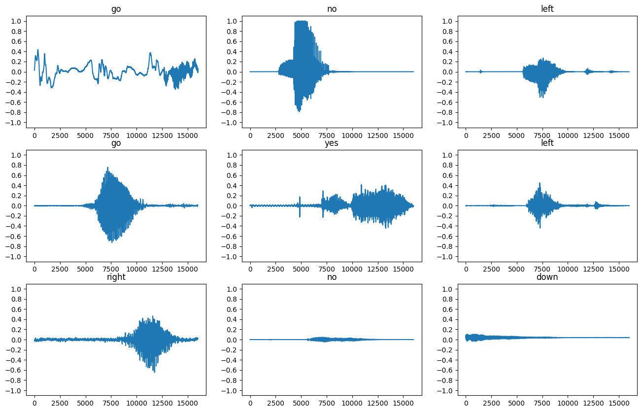
ลองพล็อตรูปคลื่นเสียงสองสามแบบ:
rows = 3
cols = 3
n = rows * cols
fig, axes = plt.subplots(rows, cols, figsize=(10, 12))

for i, (audio, label) in enumerate(waveform_ds.take(n)):
  r = i // cols
  c = i % cols
  ax = axes[r][c]
  ax.plot(audio.numpy())
  ax.set_yticks(np.arange(-1.2, 1.2, 0.2))
  label = label.numpy().decode('utf-8')
  ax.set_title(label)

plt.show()
แปลงรูปคลื่นเป็นสเปกโตรแกรม
รูปคลื่นในชุดข้อมูลจะแสดงในโดเมนเวลา ถัดไป คุณจะแปลงรูปคลื่นจากสัญญาณโดเมนเวลาเป็นสัญญาณโดเมนความถี่เวลาโดยคำนวณการ แปลงฟูเรียร์เวลาสั้น (STFT) เพื่อแปลงรูปคลื่นเป็น สเปกตรัม ซึ่งแสดงการเปลี่ยนแปลงความถี่เมื่อเวลาผ่านไปและสามารถ แสดงเป็นภาพ 2 มิติ คุณจะป้อนภาพสเปกโตรแกรมลงในโครงข่ายประสาทเทียมเพื่อฝึกโมเดล
การแปลงฟูริเยร์ ( tf.signal.fft ) แปลงสัญญาณเป็นความถี่ส่วนประกอบ แต่สูญเสียข้อมูลตลอดเวลา ในการเปรียบเทียบ STFT ( tf.signal.stft ) แบ่งสัญญาณออกเป็นหน้าต่างเวลาและเรียกใช้การแปลงฟูริเยร์ในแต่ละหน้าต่าง เก็บข้อมูลเวลาบางส่วน และส่งคืนเมตริกซ์ 2D ที่คุณสามารถเรียกใช้การบิดแบบมาตรฐานได้
สร้างฟังก์ชันยูทิลิตี้สำหรับการแปลงรูปคลื่นเป็นสเปกโตรแกรม:
- รูปคลื่นต้องมีความยาวเท่ากัน ดังนั้นเมื่อคุณแปลงเป็นสเปกโตรแกรม ผลลัพธ์จะมีขนาดใกล้เคียงกัน ซึ่งสามารถทำได้โดยเพียงแค่ใส่คลิปเสียงที่สั้นกว่าหนึ่งวินาทีเป็นศูนย์ (โดยใช้
tf.zeros) - เมื่อเรียก
tf.signal.stftให้เลือกพารามิเตอร์frame_lengthและframe_stepเพื่อให้ "image" ของสเปกโตรแกรมที่สร้างขึ้นนั้นเกือบจะเป็นสี่เหลี่ยมจัตุรัส สำหรับข้อมูลเพิ่มเติมเกี่ยวกับตัวเลือกพารามิเตอร์ STFT โปรดดู วิดีโอ Coursera เกี่ยวกับการประมวลผลสัญญาณเสียงและ STFT - STFT จะสร้างอาร์เรย์ของจำนวนเชิงซ้อนที่แสดงขนาดและเฟส อย่างไรก็ตาม ในบทช่วยสอนนี้ คุณจะใช้เฉพาะขนาด ซึ่งคุณสามารถได้รับโดยการใช้
tf.absกับผลลัพธ์ของtf.signal.stft
def get_spectrogram(waveform):
  # Zero-padding for an audio waveform with less than 16,000 samples.
  input_len = 16000
  waveform = waveform[:input_len]
  zero_padding = tf.zeros(
      [16000] - tf.shape(waveform),
      dtype=tf.float32)
  # Cast the waveform tensors' dtype to float32.
  waveform = tf.cast(waveform, dtype=tf.float32)
  # Concatenate the waveform with `zero_padding`, which ensures all audio
  # clips are of the same length.
  equal_length = tf.concat([waveform, zero_padding], 0)
  # Convert the waveform to a spectrogram via a STFT.
  spectrogram = tf.signal.stft(
      equal_length, frame_length=255, frame_step=128)
  # Obtain the magnitude of the STFT.
  spectrogram = tf.abs(spectrogram)
  # Add a `channels` dimension, so that the spectrogram can be used
  # as image-like input data with convolution layers (which expect
  # shape (`batch_size`, `height`, `width`, `channels`).
  spectrogram = spectrogram[..., tf.newaxis]
  return spectrogram
ต่อไป เริ่มสำรวจข้อมูล พิมพ์รูปร่างของรูปคลื่นเทนเซอร์ของตัวอย่างหนึ่งและสเปกโตรแกรมที่เกี่ยวข้อง แล้วเล่นเสียงต้นฉบับ:
for waveform, label in waveform_ds.take(1):
  label = label.numpy().decode('utf-8')
  spectrogram = get_spectrogram(waveform)

print('Label:', label)
print('Waveform shape:', waveform.shape)
print('Spectrogram shape:', spectrogram.shape)
print('Audio playback')
display.display(display.Audio(waveform, rate=16000))
Label: yes
Waveform shape: (16000,)
Spectrogram shape: (124, 129, 1)
Audio playback
ตอนนี้ กำหนดฟังก์ชันสำหรับแสดงสเปกโตรแกรม:
def plot_spectrogram(spectrogram, ax):
  if len(spectrogram.shape) > 2:
    assert len(spectrogram.shape) == 3
    spectrogram = np.squeeze(spectrogram, axis=-1)
  # Convert the frequencies to log scale and transpose, so that the time is
  # represented on the x-axis (columns).
  # Add an epsilon to avoid taking a log of zero.
  log_spec = np.log(spectrogram.T + np.finfo(float).eps)
  height = log_spec.shape[0]
  width = log_spec.shape[1]
  X = np.linspace(0, np.size(spectrogram), num=width, dtype=int)
  Y = range(height)
  ax.pcolormesh(X, Y, log_spec)
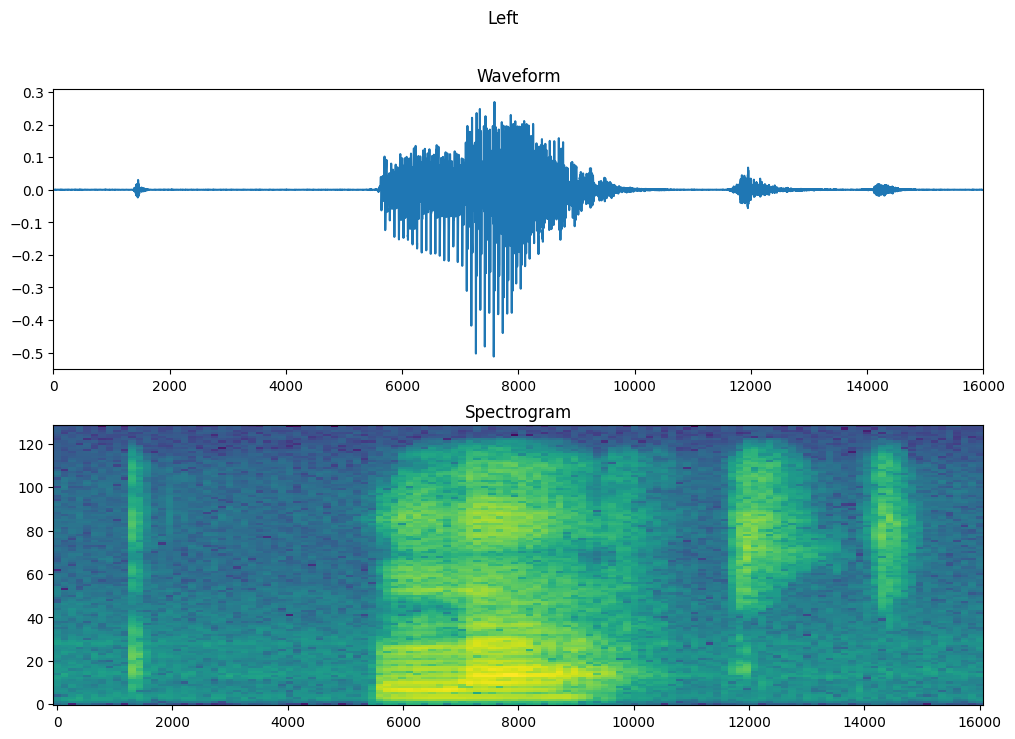
พล็อตรูปคลื่นของตัวอย่างเมื่อเวลาผ่านไปและสเปกโตรแกรมที่เกี่ยวข้อง (ความถี่เมื่อเวลาผ่านไป):
fig, axes = plt.subplots(2, figsize=(12, 8))
timescale = np.arange(waveform.shape[0])
axes[0].plot(timescale, waveform.numpy())
axes[0].set_title('Waveform')
axes[0].set_xlim([0, 16000])

plot_spectrogram(spectrogram.numpy(), axes[1])
axes[1].set_title('Spectrogram')
plt.show()
ตอนนี้ กำหนดฟังก์ชันที่แปลงชุดข้อมูลรูปคลื่นเป็นสเปกโตรแกรมและป้ายกำกับที่เกี่ยวข้องเป็น ID จำนวนเต็ม:
def get_spectrogram_and_label_id(audio, label):
  spectrogram = get_spectrogram(audio)
  label_id = tf.argmax(label == commands)
  return spectrogram, label_id
แม get_spectrogram_and_label_id ระหว่างองค์ประกอบของชุดข้อมูลด้วย Dataset.map :
spectrogram_ds = waveform_ds.map(
  map_func=get_spectrogram_and_label_id,
  num_parallel_calls=AUTOTUNE)
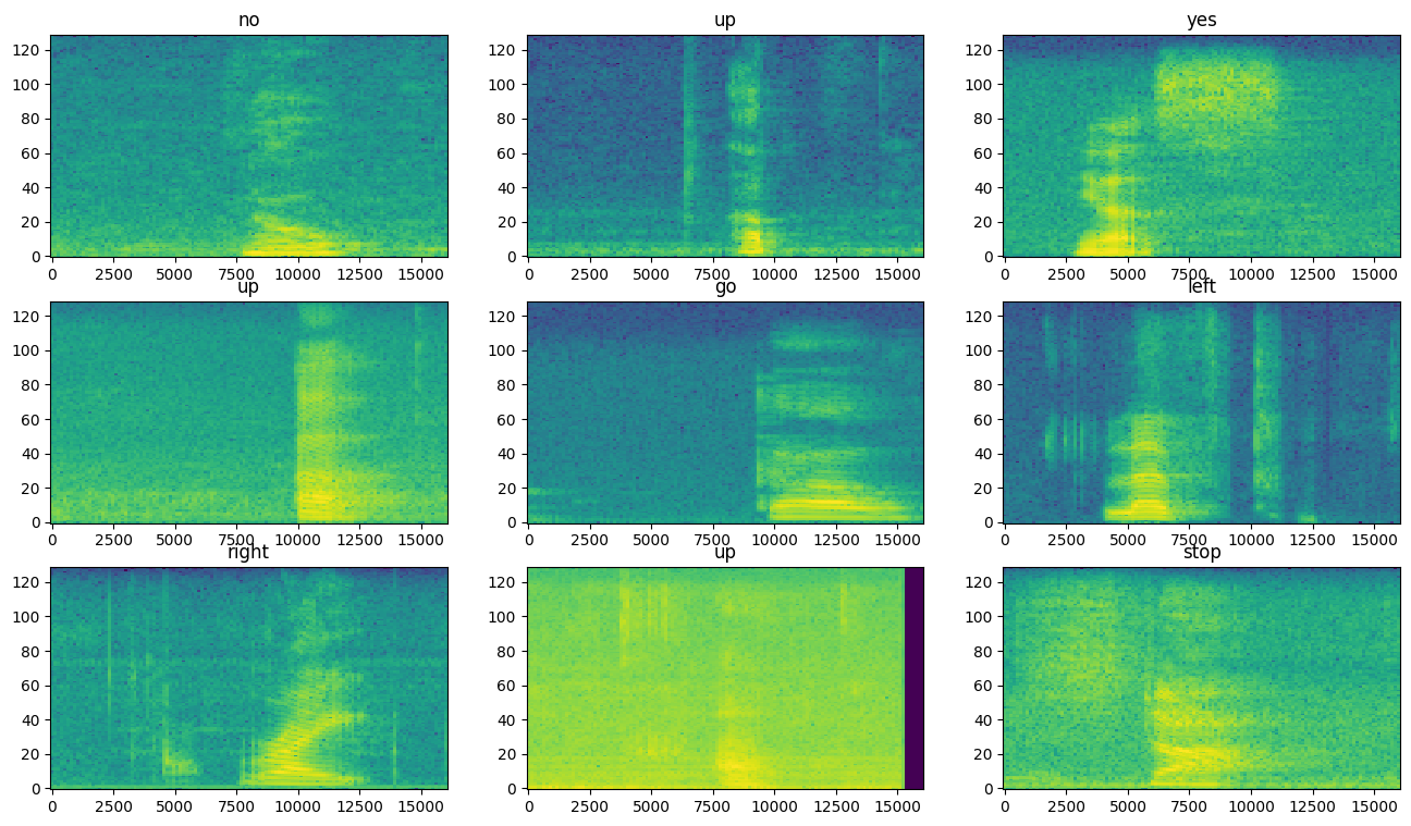
ตรวจสอบสเปกโตรแกรมสำหรับตัวอย่างต่างๆ ของชุดข้อมูล:
rows = 3
cols = 3
n = rows*cols
fig, axes = plt.subplots(rows, cols, figsize=(10, 10))

for i, (spectrogram, label_id) in enumerate(spectrogram_ds.take(n)):
  r = i // cols
  c = i % cols
  ax = axes[r][c]
  plot_spectrogram(spectrogram.numpy(), ax)
  ax.set_title(commands[label_id.numpy()])
  ax.axis('off')

plt.show()
สร้างและฝึกโมเดล
ทำซ้ำชุดการฝึกประมวลผลล่วงหน้าในชุดตรวจสอบและชุดทดสอบ:
def preprocess_dataset(files):
  files_ds = tf.data.Dataset.from_tensor_slices(files)
  output_ds = files_ds.map(
      map_func=get_waveform_and_label,
      num_parallel_calls=AUTOTUNE)
  output_ds = output_ds.map(
      map_func=get_spectrogram_and_label_id,
      num_parallel_calls=AUTOTUNE)
  return output_ds
train_ds = spectrogram_ds
val_ds = preprocess_dataset(val_files)
test_ds = preprocess_dataset(test_files)
ชุดการฝึกและการตรวจสอบความถูกต้องสำหรับการฝึกแบบจำลอง:
batch_size = 64
train_ds = train_ds.batch(batch_size)
val_ds = val_ds.batch(batch_size)
เพิ่มการดำเนินการ Dataset.cache และ Dataset.prefetch เพื่อลดเวลาแฝงในการอ่านขณะฝึกโมเดล:
train_ds = train_ds.cache().prefetch(AUTOTUNE)
val_ds = val_ds.cache().prefetch(AUTOTUNE)
สำหรับโมเดลนี้ คุณจะใช้โครงข่ายประสาทเทียมแบบง่าย (CNN) เนื่องจากคุณได้แปลงไฟล์เสียงเป็นภาพสเปกโตรแกรม
โมเดล tf.keras.Sequential ของคุณจะใช้เลเยอร์การประมวลผลล่วงหน้าของ Keras ต่อไปนี้:
-
tf.keras.layers.Resizing: เพื่อ downsample อินพุตเพื่อให้โมเดลสามารถฝึกได้เร็วขึ้น -
tf.keras.layers.Normalization: เพื่อทำให้แต่ละพิกเซลในรูปภาพเป็นมาตรฐานตามค่าเฉลี่ยและค่าเบี่ยงเบนมาตรฐาน
สำหรับเลเยอร์ Normalization ขั้นแรกต้องเรียกใช้วิธี adapt กับข้อมูลการฝึกเพื่อคำนวณสถิติรวม (นั่นคือ ค่าเฉลี่ยและค่าเบี่ยงเบนมาตรฐาน)
for spectrogram, _ in spectrogram_ds.take(1):
  input_shape = spectrogram.shape
print('Input shape:', input_shape)
num_labels = len(commands)

# Instantiate the `tf.keras.layers.Normalization` layer.
norm_layer = layers.Normalization()
# Fit the state of the layer to the spectrograms
# with `Normalization.adapt`.
norm_layer.adapt(data=spectrogram_ds.map(map_func=lambda spec, label: spec))

model = models.Sequential([
    layers.Input(shape=input_shape),
    # Downsample the input.
    layers.Resizing(32, 32),
    # Normalize.
    norm_layer,
    layers.Conv2D(32, 3, activation='relu'),
    layers.Conv2D(64, 3, activation='relu'),
    layers.MaxPooling2D(),
    layers.Dropout(0.25),
    layers.Flatten(),
    layers.Dense(128, activation='relu'),
    layers.Dropout(0.5),
    layers.Dense(num_labels),
])

model.summary()
Input shape: (124, 129, 1)
Model: "sequential"
_________________________________________________________________
 Layer (type)                Output Shape              Param #
=================================================================
 resizing (Resizing)         (None, 32, 32, 1)         0

 normalization (Normalizatio  (None, 32, 32, 1)        3
 n)

 conv2d (Conv2D)             (None, 30, 30, 32)        320

 conv2d_1 (Conv2D)           (None, 28, 28, 64)        18496

 max_pooling2d (MaxPooling2D  (None, 14, 14, 64)       0
 )

 dropout (Dropout)           (None, 14, 14, 64)        0

 flatten (Flatten)           (None, 12544)             0

 dense (Dense)               (None, 128)               1605760

 dropout_1 (Dropout)         (None, 128)               0

 dense_1 (Dense)             (None, 8)                 1032

=================================================================
Total params: 1,625,611
Trainable params: 1,625,608
Non-trainable params: 3
_________________________________________________________________
กำหนดค่าโมเดล Keras ด้วยเครื่องมือเพิ่มประสิทธิภาพ Adam และการสูญเสียเอนโทรปีแบบไขว้:
model.compile(
    optimizer=tf.keras.optimizers.Adam(),
    loss=tf.keras.losses.SparseCategoricalCrossentropy(from_logits=True),
    metrics=['accuracy'],
)
ฝึกโมเดลมากกว่า 10 ยุคเพื่อจุดประสงค์ในการสาธิต:
EPOCHS = 10
history = model.fit(
    train_ds,
    validation_data=val_ds,
    epochs=EPOCHS,
    callbacks=tf.keras.callbacks.EarlyStopping(verbose=1, patience=2),
)
Epoch 1/10
100/100 [==============================] - 6s 41ms/step - loss: 1.7503 - accuracy: 0.3630 - val_loss: 1.2850 - val_accuracy: 0.5763
Epoch 2/10
100/100 [==============================] - 0s 5ms/step - loss: 1.2101 - accuracy: 0.5698 - val_loss: 0.9314 - val_accuracy: 0.6913
Epoch 3/10
100/100 [==============================] - 0s 5ms/step - loss: 0.9336 - accuracy: 0.6703 - val_loss: 0.7529 - val_accuracy: 0.7325
Epoch 4/10
100/100 [==============================] - 0s 5ms/step - loss: 0.7503 - accuracy: 0.7397 - val_loss: 0.6721 - val_accuracy: 0.7713
Epoch 5/10
100/100 [==============================] - 0s 5ms/step - loss: 0.6367 - accuracy: 0.7741 - val_loss: 0.6061 - val_accuracy: 0.7975
Epoch 6/10
100/100 [==============================] - 0s 5ms/step - loss: 0.5650 - accuracy: 0.7987 - val_loss: 0.5489 - val_accuracy: 0.8125
Epoch 7/10
100/100 [==============================] - 0s 5ms/step - loss: 0.5099 - accuracy: 0.8183 - val_loss: 0.5344 - val_accuracy: 0.8238
Epoch 8/10
100/100 [==============================] - 0s 5ms/step - loss: 0.4560 - accuracy: 0.8392 - val_loss: 0.5194 - val_accuracy: 0.8288
Epoch 9/10
100/100 [==============================] - 0s 5ms/step - loss: 0.4101 - accuracy: 0.8547 - val_loss: 0.4809 - val_accuracy: 0.8388
Epoch 10/10
100/100 [==============================] - 0s 5ms/step - loss: 0.3905 - accuracy: 0.8589 - val_loss: 0.4973 - val_accuracy: 0.8363
ตัวยึดตำแหน่ง33
เรามาพลอตกราฟการฝึกอบรมและการสูญเสียการตรวจสอบเพื่อตรวจสอบว่าโมเดลของคุณได้รับการปรับปรุงระหว่างการฝึกอย่างไร:
metrics = history.history
plt.plot(history.epoch, metrics['loss'], metrics['val_loss'])
plt.legend(['loss', 'val_loss'])
plt.show()

ประเมินประสิทธิภาพของแบบจำลอง
เรียกใช้แบบจำลองในชุดทดสอบและตรวจสอบประสิทธิภาพของแบบจำลอง:
test_audio = []
test_labels = []

for audio, label in test_ds:
  test_audio.append(audio.numpy())
  test_labels.append(label.numpy())

test_audio = np.array(test_audio)
test_labels = np.array(test_labels)
y_pred = np.argmax(model.predict(test_audio), axis=1)
y_true = test_labels

test_acc = sum(y_pred == y_true) / len(y_true)
print(f'Test set accuracy: {test_acc:.0%}')
Test set accuracy: 85%
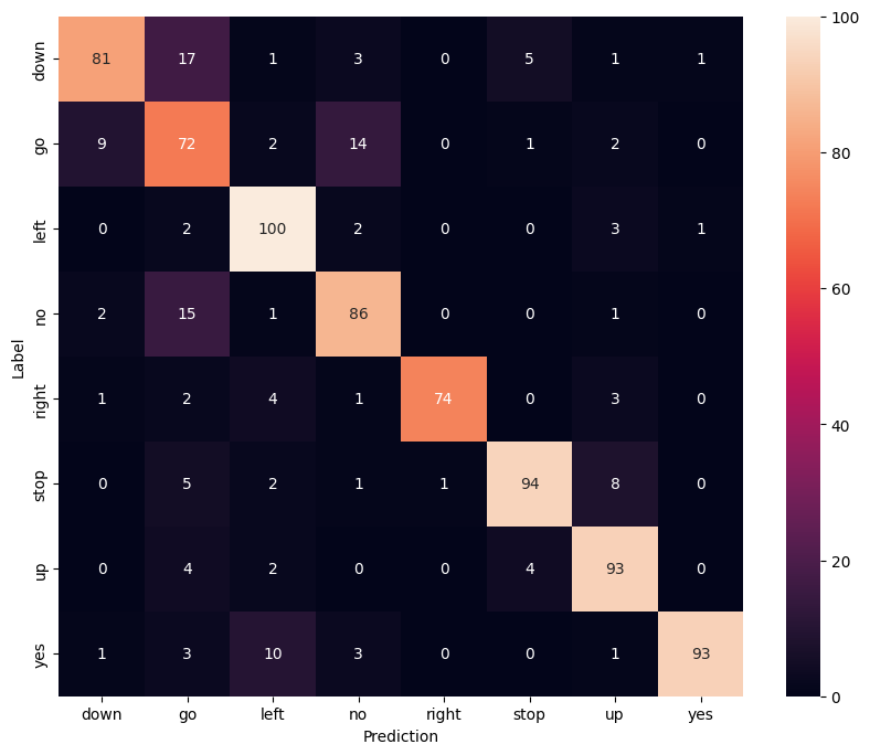
แสดงเมทริกซ์ความสับสน
ใช้ เมทริกซ์ความสับสน เพื่อตรวจสอบว่าโมเดลจำแนกแต่ละคำสั่งในชุดการทดสอบได้ดีเพียงใด:
confusion_mtx = tf.math.confusion_matrix(y_true, y_pred)
plt.figure(figsize=(10, 8))
sns.heatmap(confusion_mtx,
            xticklabels=commands,
            yticklabels=commands,
            annot=True, fmt='g')
plt.xlabel('Prediction')
plt.ylabel('Label')
plt.show()
เรียกใช้การอนุมานบนไฟล์เสียง
สุดท้าย ตรวจสอบเอาต์พุตการคาดคะเนของโมเดลโดยใช้ไฟล์เสียงอินพุตของใครบางคนที่พูดว่า "ไม่" โมเดลของคุณทำงานได้ดีเพียงใด?
sample_file = data_dir/'no/01bb6a2a_nohash_0.wav'

sample_ds = preprocess_dataset([str(sample_file)])

for spectrogram, label in sample_ds.batch(1):
  prediction = model(spectrogram)
  plt.bar(commands, tf.nn.softmax(prediction[0]))
  plt.title(f'Predictions for "{commands[label[0]]}"')
  plt.show()
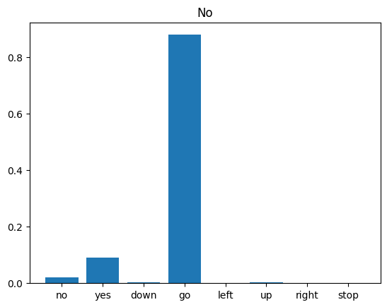
ตามที่ผลลัพธ์แนะนำ โมเดลของคุณควรรู้จักคำสั่งเสียงเป็น "ไม่"
ขั้นตอนถัดไป
บทช่วยสอนนี้สาธิตวิธีดำเนินการจำแนกเสียงอย่างง่าย/การรู้จำคำพูดอัตโนมัติโดยใช้โครงข่ายประสาทเทียมที่มี TensorFlow และ Python หากต้องการเรียนรู้เพิ่มเติม ให้พิจารณาแหล่งข้อมูลต่อไปนี้:
- การ จัดหมวดหมู่เสียงด้วยบทช่วยสอน YAMNet แสดงวิธีใช้การเรียนรู้การถ่ายโอนสำหรับการจัดประเภทเสียง
- สมุดบันทึกจาก ความท้าทายการรู้จำเสียงพูด TensorFlow ของ Kaggle
- TensorFlow.js - การรู้จำเสียงโดยใช้ Codelab การเรียนรู้การถ่ายโอนจะ สอนวิธีสร้างเว็บแอปเชิงโต้ตอบของคุณเองสำหรับการจัดประเภทเสียง
- บทช่วยสอนเกี่ยวกับการเรียนรู้เชิงลึกสำหรับการดึงข้อมูลเพลง (Choi et al., 2017) บน arXiv
- TensorFlow ยังมีการสนับสนุนเพิ่มเติมสำหรับ การเตรียมข้อมูลเสียงและการเสริม เพื่อช่วยในโครงการที่ใช้เสียงของคุณเอง
- ลองใช้ไลบรารี librosa ซึ่งเป็นแพ็คเกจ Python สำหรับการวิเคราะห์เพลงและเสียง