
|
|
|
 View source on GitHub
|
|
This tutorial introduces autoencoders with three examples: the basics, image denoising, and anomaly detection.
An autoencoder is a special type of neural network that is trained to copy its input to its output. For example, given an image of a handwritten digit, an autoencoder first encodes the image into a lower dimensional latent representation, then decodes the latent representation back to an image. An autoencoder learns to compress the data while minimizing the reconstruction error.
To learn more about autoencoders, please consider reading chapter 14 from Deep Learning by Ian Goodfellow, Yoshua Bengio, and Aaron Courville.
Import TensorFlow and other libraries
import matplotlib.pyplot as plt
import numpy as np
import pandas as pd
import tensorflow as tf

from sklearn.metrics import accuracy_score, precision_score, recall_score
from sklearn.model_selection import train_test_split
from tensorflow.keras import layers, losses
from tensorflow.keras.datasets import fashion_mnist
from tensorflow.keras.models import Model
2024-08-16 05:08:24.454969: E external/local_xla/xla/stream_executor/cuda/cuda_fft.cc:485] Unable to register cuFFT factory: Attempting to register factory for plugin cuFFT when one has already been registered
2024-08-16 05:08:24.475836: E external/local_xla/xla/stream_executor/cuda/cuda_dnn.cc:8454] Unable to register cuDNN factory: Attempting to register factory for plugin cuDNN when one has already been registered
2024-08-16 05:08:24.482184: E external/local_xla/xla/stream_executor/cuda/cuda_blas.cc:1452] Unable to register cuBLAS factory: Attempting to register factory for plugin cuBLAS when one has already been registered
Load the dataset
To start, you will train the basic autoencoder using the Fashion MNIST dataset. Each image in this dataset is 28x28 pixels.
(x_train, _), (x_test, _) = fashion_mnist.load_data()

x_train = x_train.astype('float32') / 255.
x_test = x_test.astype('float32') / 255.

print (x_train.shape)
print (x_test.shape)
(60000, 28, 28)
(10000, 28, 28)
First example: Basic autoencoder
Define an autoencoder with two Dense layers: an encoder, which compresses the images into a 64 dimensional latent vector, and a decoder, that reconstructs the original image from the latent space.
To define your model, use the Keras Model Subclassing API.
class Autoencoder(Model):
  def __init__(self, latent_dim, shape):
    super(Autoencoder, self).__init__()
    self.latent_dim = latent_dim
    self.shape = shape
    self.encoder = tf.keras.Sequential([
      layers.Flatten(),
      layers.Dense(latent_dim, activation='relu'),
    ])
    self.decoder = tf.keras.Sequential([
      layers.Dense(tf.math.reduce_prod(shape).numpy(), activation='sigmoid'),
      layers.Reshape(shape)
    ])

  def call(self, x):
    encoded = self.encoder(x)
    decoded = self.decoder(encoded)
    return decoded


shape = x_test.shape[1:]
latent_dim = 64
autoencoder = Autoencoder(latent_dim, shape)
WARNING: All log messages before absl::InitializeLog() is called are written to STDERR
I0000 00:00:1723784907.495092  160375 cuda_executor.cc:1015] successful NUMA node read from SysFS had negative value (-1), but there must be at least one NUMA node, so returning NUMA node zero. See more at https://github.com/torvalds/linux/blob/v6.0/Documentation/ABI/testing/sysfs-bus-pci#L344-L355
I0000 00:00:1723784907.498985  160375 cuda_executor.cc:1015] successful NUMA node read from SysFS had negative value (-1), but there must be at least one NUMA node, so returning NUMA node zero. See more at https://github.com/torvalds/linux/blob/v6.0/Documentation/ABI/testing/sysfs-bus-pci#L344-L355
I0000 00:00:1723784907.502627  160375 cuda_executor.cc:1015] successful NUMA node read from SysFS had negative value (-1), but there must be at least one NUMA node, so returning NUMA node zero. See more at https://github.com/torvalds/linux/blob/v6.0/Documentation/ABI/testing/sysfs-bus-pci#L344-L355
I0000 00:00:1723784907.506226  160375 cuda_executor.cc:1015] successful NUMA node read from SysFS had negative value (-1), but there must be at least one NUMA node, so returning NUMA node zero. See more at https://github.com/torvalds/linux/blob/v6.0/Documentation/ABI/testing/sysfs-bus-pci#L344-L355
I0000 00:00:1723784907.518853  160375 cuda_executor.cc:1015] successful NUMA node read from SysFS had negative value (-1), but there must be at least one NUMA node, so returning NUMA node zero. See more at https://github.com/torvalds/linux/blob/v6.0/Documentation/ABI/testing/sysfs-bus-pci#L344-L355
I0000 00:00:1723784907.522303  160375 cuda_executor.cc:1015] successful NUMA node read from SysFS had negative value (-1), but there must be at least one NUMA node, so returning NUMA node zero. See more at https://github.com/torvalds/linux/blob/v6.0/Documentation/ABI/testing/sysfs-bus-pci#L344-L355
I0000 00:00:1723784907.525756  160375 cuda_executor.cc:1015] successful NUMA node read from SysFS had negative value (-1), but there must be at least one NUMA node, so returning NUMA node zero. See more at https://github.com/torvalds/linux/blob/v6.0/Documentation/ABI/testing/sysfs-bus-pci#L344-L355
I0000 00:00:1723784907.529169  160375 cuda_executor.cc:1015] successful NUMA node read from SysFS had negative value (-1), but there must be at least one NUMA node, so returning NUMA node zero. See more at https://github.com/torvalds/linux/blob/v6.0/Documentation/ABI/testing/sysfs-bus-pci#L344-L355
I0000 00:00:1723784907.532506  160375 cuda_executor.cc:1015] successful NUMA node read from SysFS had negative value (-1), but there must be at least one NUMA node, so returning NUMA node zero. See more at https://github.com/torvalds/linux/blob/v6.0/Documentation/ABI/testing/sysfs-bus-pci#L344-L355
I0000 00:00:1723784907.536023  160375 cuda_executor.cc:1015] successful NUMA node read from SysFS had negative value (-1), but there must be at least one NUMA node, so returning NUMA node zero. See more at https://github.com/torvalds/linux/blob/v6.0/Documentation/ABI/testing/sysfs-bus-pci#L344-L355
I0000 00:00:1723784907.539501  160375 cuda_executor.cc:1015] successful NUMA node read from SysFS had negative value (-1), but there must be at least one NUMA node, so returning NUMA node zero. See more at https://github.com/torvalds/linux/blob/v6.0/Documentation/ABI/testing/sysfs-bus-pci#L344-L355
I0000 00:00:1723784907.542895  160375 cuda_executor.cc:1015] successful NUMA node read from SysFS had negative value (-1), but there must be at least one NUMA node, so returning NUMA node zero. See more at https://github.com/torvalds/linux/blob/v6.0/Documentation/ABI/testing/sysfs-bus-pci#L344-L355
I0000 00:00:1723784908.772373  160375 cuda_executor.cc:1015] successful NUMA node read from SysFS had negative value (-1), but there must be at least one NUMA node, so returning NUMA node zero. See more at https://github.com/torvalds/linux/blob/v6.0/Documentation/ABI/testing/sysfs-bus-pci#L344-L355
I0000 00:00:1723784908.774589  160375 cuda_executor.cc:1015] successful NUMA node read from SysFS had negative value (-1), but there must be at least one NUMA node, so returning NUMA node zero. See more at https://github.com/torvalds/linux/blob/v6.0/Documentation/ABI/testing/sysfs-bus-pci#L344-L355
I0000 00:00:1723784908.776554  160375 cuda_executor.cc:1015] successful NUMA node read from SysFS had negative value (-1), but there must be at least one NUMA node, so returning NUMA node zero. See more at https://github.com/torvalds/linux/blob/v6.0/Documentation/ABI/testing/sysfs-bus-pci#L344-L355
I0000 00:00:1723784908.778641  160375 cuda_executor.cc:1015] successful NUMA node read from SysFS had negative value (-1), but there must be at least one NUMA node, so returning NUMA node zero. See more at https://github.com/torvalds/linux/blob/v6.0/Documentation/ABI/testing/sysfs-bus-pci#L344-L355
I0000 00:00:1723784908.780679  160375 cuda_executor.cc:1015] successful NUMA node read from SysFS had negative value (-1), but there must be at least one NUMA node, so returning NUMA node zero. See more at https://github.com/torvalds/linux/blob/v6.0/Documentation/ABI/testing/sysfs-bus-pci#L344-L355
I0000 00:00:1723784908.782717  160375 cuda_executor.cc:1015] successful NUMA node read from SysFS had negative value (-1), but there must be at least one NUMA node, so returning NUMA node zero. See more at https://github.com/torvalds/linux/blob/v6.0/Documentation/ABI/testing/sysfs-bus-pci#L344-L355
I0000 00:00:1723784908.784577  160375 cuda_executor.cc:1015] successful NUMA node read from SysFS had negative value (-1), but there must be at least one NUMA node, so returning NUMA node zero. See more at https://github.com/torvalds/linux/blob/v6.0/Documentation/ABI/testing/sysfs-bus-pci#L344-L355
I0000 00:00:1723784908.786661  160375 cuda_executor.cc:1015] successful NUMA node read from SysFS had negative value (-1), but there must be at least one NUMA node, so returning NUMA node zero. See more at https://github.com/torvalds/linux/blob/v6.0/Documentation/ABI/testing/sysfs-bus-pci#L344-L355
I0000 00:00:1723784908.788966  160375 cuda_executor.cc:1015] successful NUMA node read from SysFS had negative value (-1), but there must be at least one NUMA node, so returning NUMA node zero. See more at https://github.com/torvalds/linux/blob/v6.0/Documentation/ABI/testing/sysfs-bus-pci#L344-L355
I0000 00:00:1723784908.791004  160375 cuda_executor.cc:1015] successful NUMA node read from SysFS had negative value (-1), but there must be at least one NUMA node, so returning NUMA node zero. See more at https://github.com/torvalds/linux/blob/v6.0/Documentation/ABI/testing/sysfs-bus-pci#L344-L355
I0000 00:00:1723784908.792858  160375 cuda_executor.cc:1015] successful NUMA node read from SysFS had negative value (-1), but there must be at least one NUMA node, so returning NUMA node zero. See more at https://github.com/torvalds/linux/blob/v6.0/Documentation/ABI/testing/sysfs-bus-pci#L344-L355
I0000 00:00:1723784908.795056  160375 cuda_executor.cc:1015] successful NUMA node read from SysFS had negative value (-1), but there must be at least one NUMA node, so returning NUMA node zero. See more at https://github.com/torvalds/linux/blob/v6.0/Documentation/ABI/testing/sysfs-bus-pci#L344-L355
I0000 00:00:1723784908.833540  160375 cuda_executor.cc:1015] successful NUMA node read from SysFS had negative value (-1), but there must be at least one NUMA node, so returning NUMA node zero. See more at https://github.com/torvalds/linux/blob/v6.0/Documentation/ABI/testing/sysfs-bus-pci#L344-L355
I0000 00:00:1723784908.835672  160375 cuda_executor.cc:1015] successful NUMA node read from SysFS had negative value (-1), but there must be at least one NUMA node, so returning NUMA node zero. See more at https://github.com/torvalds/linux/blob/v6.0/Documentation/ABI/testing/sysfs-bus-pci#L344-L355
I0000 00:00:1723784908.837578  160375 cuda_executor.cc:1015] successful NUMA node read from SysFS had negative value (-1), but there must be at least one NUMA node, so returning NUMA node zero. See more at https://github.com/torvalds/linux/blob/v6.0/Documentation/ABI/testing/sysfs-bus-pci#L344-L355
I0000 00:00:1723784908.839614  160375 cuda_executor.cc:1015] successful NUMA node read from SysFS had negative value (-1), but there must be at least one NUMA node, so returning NUMA node zero. See more at https://github.com/torvalds/linux/blob/v6.0/Documentation/ABI/testing/sysfs-bus-pci#L344-L355
I0000 00:00:1723784908.841487  160375 cuda_executor.cc:1015] successful NUMA node read from SysFS had negative value (-1), but there must be at least one NUMA node, so returning NUMA node zero. See more at https://github.com/torvalds/linux/blob/v6.0/Documentation/ABI/testing/sysfs-bus-pci#L344-L355
I0000 00:00:1723784908.843549  160375 cuda_executor.cc:1015] successful NUMA node read from SysFS had negative value (-1), but there must be at least one NUMA node, so returning NUMA node zero. See more at https://github.com/torvalds/linux/blob/v6.0/Documentation/ABI/testing/sysfs-bus-pci#L344-L355
I0000 00:00:1723784908.845399  160375 cuda_executor.cc:1015] successful NUMA node read from SysFS had negative value (-1), but there must be at least one NUMA node, so returning NUMA node zero. See more at https://github.com/torvalds/linux/blob/v6.0/Documentation/ABI/testing/sysfs-bus-pci#L344-L355
I0000 00:00:1723784908.847401  160375 cuda_executor.cc:1015] successful NUMA node read from SysFS had negative value (-1), but there must be at least one NUMA node, so returning NUMA node zero. See more at https://github.com/torvalds/linux/blob/v6.0/Documentation/ABI/testing/sysfs-bus-pci#L344-L355
I0000 00:00:1723784908.849242  160375 cuda_executor.cc:1015] successful NUMA node read from SysFS had negative value (-1), but there must be at least one NUMA node, so returning NUMA node zero. See more at https://github.com/torvalds/linux/blob/v6.0/Documentation/ABI/testing/sysfs-bus-pci#L344-L355
I0000 00:00:1723784908.851783  160375 cuda_executor.cc:1015] successful NUMA node read from SysFS had negative value (-1), but there must be at least one NUMA node, so returning NUMA node zero. See more at https://github.com/torvalds/linux/blob/v6.0/Documentation/ABI/testing/sysfs-bus-pci#L344-L355
I0000 00:00:1723784908.854229  160375 cuda_executor.cc:1015] successful NUMA node read from SysFS had negative value (-1), but there must be at least one NUMA node, so returning NUMA node zero. See more at https://github.com/torvalds/linux/blob/v6.0/Documentation/ABI/testing/sysfs-bus-pci#L344-L355
I0000 00:00:1723784908.856641  160375 cuda_executor.cc:1015] successful NUMA node read from SysFS had negative value (-1), but there must be at least one NUMA node, so returning NUMA node zero. See more at https://github.com/torvalds/linux/blob/v6.0/Documentation/ABI/testing/sysfs-bus-pci#L344-L355
autoencoder.compile(optimizer='adam', loss=losses.MeanSquaredError())
Train the model using x_train as both the input and the target. The encoder will learn to compress the dataset from 784 dimensions to the latent space, and the decoder will learn to reconstruct the original images.
.
autoencoder.fit(x_train, x_train,
                epochs=10,
                shuffle=True,
                validation_data=(x_test, x_test))
Epoch 1/10
WARNING: All log messages before absl::InitializeLog() is called are written to STDERR
I0000 00:00:1723784911.543932  160540 service.cc:146] XLA service 0x7f8910006f20 initialized for platform CUDA (this does not guarantee that XLA will be used). Devices:
I0000 00:00:1723784911.543965  160540 service.cc:154]   StreamExecutor device (0): Tesla T4, Compute Capability 7.5
I0000 00:00:1723784911.543969  160540 service.cc:154]   StreamExecutor device (1): Tesla T4, Compute Capability 7.5
I0000 00:00:1723784911.543973  160540 service.cc:154]   StreamExecutor device (2): Tesla T4, Compute Capability 7.5
I0000 00:00:1723784911.543976  160540 service.cc:154]   StreamExecutor device (3): Tesla T4, Compute Capability 7.5
137/1875 ━━━━━━━━━━━━━━━━━━━━ 1s 1ms/step - loss: 0.1008
I0000 00:00:1723784912.197500  160540 device_compiler.h:188] Compiled cluster using XLA!  This line is logged at most once for the lifetime of the process.
1875/1875 ━━━━━━━━━━━━━━━━━━━━ 5s 2ms/step - loss: 0.0402 - val_loss: 0.0134
Epoch 2/10
1875/1875 ━━━━━━━━━━━━━━━━━━━━ 2s 1ms/step - loss: 0.0124 - val_loss: 0.0106
Epoch 3/10
1875/1875 ━━━━━━━━━━━━━━━━━━━━ 2s 1ms/step - loss: 0.0104 - val_loss: 0.0098
Epoch 4/10
1875/1875 ━━━━━━━━━━━━━━━━━━━━ 2s 1ms/step - loss: 0.0097 - val_loss: 0.0095
Epoch 5/10
1875/1875 ━━━━━━━━━━━━━━━━━━━━ 2s 1ms/step - loss: 0.0093 - val_loss: 0.0092
Epoch 6/10
1875/1875 ━━━━━━━━━━━━━━━━━━━━ 2s 1ms/step - loss: 0.0092 - val_loss: 0.0091
Epoch 7/10
1875/1875 ━━━━━━━━━━━━━━━━━━━━ 2s 1ms/step - loss: 0.0090 - val_loss: 0.0090
Epoch 8/10
1875/1875 ━━━━━━━━━━━━━━━━━━━━ 2s 1ms/step - loss: 0.0089 - val_loss: 0.0089
Epoch 9/10
1875/1875 ━━━━━━━━━━━━━━━━━━━━ 2s 1ms/step - loss: 0.0089 - val_loss: 0.0089
Epoch 10/10
1875/1875 ━━━━━━━━━━━━━━━━━━━━ 2s 1ms/step - loss: 0.0088 - val_loss: 0.0090
<keras.src.callbacks.history.History at 0x7f8ac42a3460>
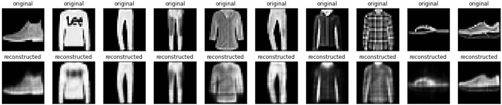
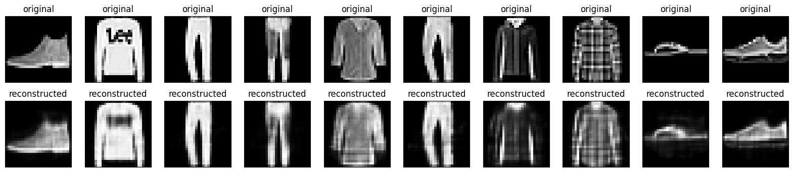
Now that the model is trained, let's test it by encoding and decoding images from the test set.
encoded_imgs = autoencoder.encoder(x_test).numpy()
decoded_imgs = autoencoder.decoder(encoded_imgs).numpy()
n = 10
plt.figure(figsize=(20, 4))
for i in range(n):
  # display original
  ax = plt.subplot(2, n, i + 1)
  plt.imshow(x_test[i])
  plt.title("original")
  plt.gray()
  ax.get_xaxis().set_visible(False)
  ax.get_yaxis().set_visible(False)

  # display reconstruction
  ax = plt.subplot(2, n, i + 1 + n)
  plt.imshow(decoded_imgs[i])
  plt.title("reconstructed")
  plt.gray()
  ax.get_xaxis().set_visible(False)
  ax.get_yaxis().set_visible(False)
plt.show()
Second example: Image denoising
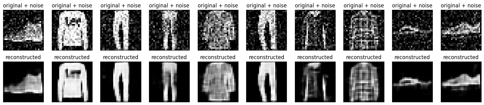
An autoencoder can also be trained to remove noise from images. In the following section, you will create a noisy version of the Fashion MNIST dataset by applying random noise to each image. You will then train an autoencoder using the noisy image as input, and the original image as the target.
Let's reimport the dataset to omit the modifications made earlier.
(x_train, _), (x_test, _) = fashion_mnist.load_data()
x_train = x_train.astype('float32') / 255.
x_test = x_test.astype('float32') / 255.

x_train = x_train[..., tf.newaxis]
x_test = x_test[..., tf.newaxis]

print(x_train.shape)
(60000, 28, 28, 1)
Adding random noise to the images
noise_factor = 0.2
x_train_noisy = x_train + noise_factor * tf.random.normal(shape=x_train.shape)
x_test_noisy = x_test + noise_factor * tf.random.normal(shape=x_test.shape)

x_train_noisy = tf.clip_by_value(x_train_noisy, clip_value_min=0., clip_value_max=1.)
x_test_noisy = tf.clip_by_value(x_test_noisy, clip_value_min=0., clip_value_max=1.)
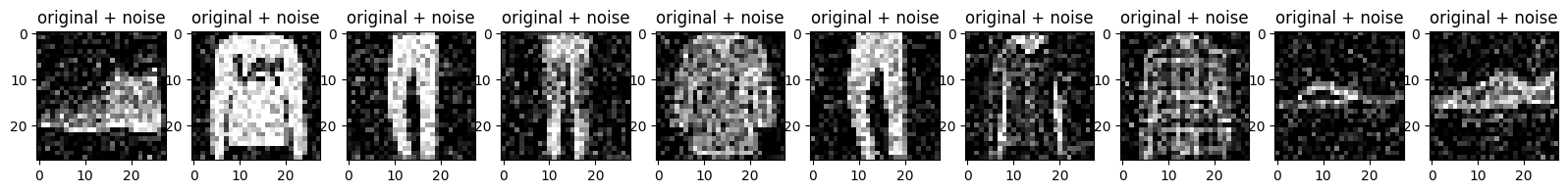
Plot the noisy images.
n = 10
plt.figure(figsize=(20, 2))
for i in range(n):
    ax = plt.subplot(1, n, i + 1)
    plt.title("original + noise")
    plt.imshow(tf.squeeze(x_test_noisy[i]))
    plt.gray()
plt.show()
Define a convolutional autoencoder
In this example, you will train a convolutional autoencoder using Conv2D layers in the encoder, and Conv2DTranspose layers in the decoder.
class Denoise(Model):
  def __init__(self):
    super(Denoise, self).__init__()
    self.encoder = tf.keras.Sequential([
      layers.Input(shape=(28, 28, 1)),
      layers.Conv2D(16, (3, 3), activation='relu', padding='same', strides=2),
      layers.Conv2D(8, (3, 3), activation='relu', padding='same', strides=2)])

    self.decoder = tf.keras.Sequential([
      layers.Conv2DTranspose(8, kernel_size=3, strides=2, activation='relu', padding='same'),
      layers.Conv2DTranspose(16, kernel_size=3, strides=2, activation='relu', padding='same'),
      layers.Conv2D(1, kernel_size=(3, 3), activation='sigmoid', padding='same')])

  def call(self, x):
    encoded = self.encoder(x)
    decoded = self.decoder(encoded)
    return decoded

autoencoder = Denoise()
autoencoder.compile(optimizer='adam', loss=losses.MeanSquaredError())
autoencoder.fit(x_train_noisy, x_train,
                epochs=10,
                shuffle=True,
                validation_data=(x_test_noisy, x_test))
Epoch 1/10
1875/1875 ━━━━━━━━━━━━━━━━━━━━ 7s 2ms/step - loss: 0.0334 - val_loss: 0.0095
Epoch 2/10
1875/1875 ━━━━━━━━━━━━━━━━━━━━ 4s 2ms/step - loss: 0.0091 - val_loss: 0.0083
Epoch 3/10
1875/1875 ━━━━━━━━━━━━━━━━━━━━ 4s 2ms/step - loss: 0.0082 - val_loss: 0.0078
Epoch 4/10
1875/1875 ━━━━━━━━━━━━━━━━━━━━ 4s 2ms/step - loss: 0.0077 - val_loss: 0.0076
Epoch 5/10
1875/1875 ━━━━━━━━━━━━━━━━━━━━ 4s 2ms/step - loss: 0.0075 - val_loss: 0.0074
Epoch 6/10
1875/1875 ━━━━━━━━━━━━━━━━━━━━ 4s 2ms/step - loss: 0.0073 - val_loss: 0.0073
Epoch 7/10
1875/1875 ━━━━━━━━━━━━━━━━━━━━ 4s 2ms/step - loss: 0.0072 - val_loss: 0.0072
Epoch 8/10
1875/1875 ━━━━━━━━━━━━━━━━━━━━ 4s 2ms/step - loss: 0.0071 - val_loss: 0.0071
Epoch 9/10
1875/1875 ━━━━━━━━━━━━━━━━━━━━ 4s 2ms/step - loss: 0.0071 - val_loss: 0.0070
Epoch 10/10
1875/1875 ━━━━━━━━━━━━━━━━━━━━ 4s 2ms/step - loss: 0.0070 - val_loss: 0.0070
<keras.src.callbacks.history.History at 0x7f8ad316bb20>
Let's take a look at a summary of the encoder. Notice how the images are downsampled from 28x28 to 7x7.
autoencoder.encoder.summary()
The decoder upsamples the images back from 7x7 to 28x28.
autoencoder.decoder.summary()
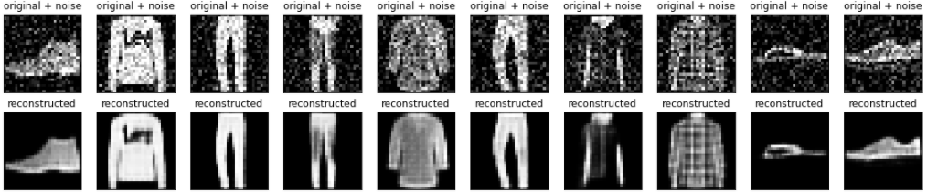
Plotting both the noisy images and the denoised images produced by the autoencoder.
encoded_imgs = autoencoder.encoder(x_test_noisy).numpy()
decoded_imgs = autoencoder.decoder(encoded_imgs).numpy()
W0000 00:00:1723784980.750910  160375 gpu_timer.cc:114] Skipping the delay kernel, measurement accuracy will be reduced
W0000 00:00:1723784980.770565  160375 gpu_timer.cc:114] Skipping the delay kernel, measurement accuracy will be reduced
W0000 00:00:1723784980.772594  160375 gpu_timer.cc:114] Skipping the delay kernel, measurement accuracy will be reduced
W0000 00:00:1723784980.774806  160375 gpu_timer.cc:114] Skipping the delay kernel, measurement accuracy will be reduced
W0000 00:00:1723784980.777004  160375 gpu_timer.cc:114] Skipping the delay kernel, measurement accuracy will be reduced
W0000 00:00:1723784980.780048  160375 gpu_timer.cc:114] Skipping the delay kernel, measurement accuracy will be reduced
W0000 00:00:1723784980.782568  160375 gpu_timer.cc:114] Skipping the delay kernel, measurement accuracy will be reduced
W0000 00:00:1723784980.785629  160375 gpu_timer.cc:114] Skipping the delay kernel, measurement accuracy will be reduced
W0000 00:00:1723784980.788932  160375 gpu_timer.cc:114] Skipping the delay kernel, measurement accuracy will be reduced
W0000 00:00:1723784980.791584  160375 gpu_timer.cc:114] Skipping the delay kernel, measurement accuracy will be reduced
W0000 00:00:1723784980.796207  160375 gpu_timer.cc:114] Skipping the delay kernel, measurement accuracy will be reduced
W0000 00:00:1723784980.799227  160375 gpu_timer.cc:114] Skipping the delay kernel, measurement accuracy will be reduced
W0000 00:00:1723784980.804537  160375 gpu_timer.cc:114] Skipping the delay kernel, measurement accuracy will be reduced
W0000 00:00:1723784980.809107  160375 gpu_timer.cc:114] Skipping the delay kernel, measurement accuracy will be reduced
W0000 00:00:1723784980.819083  160375 gpu_timer.cc:114] Skipping the delay kernel, measurement accuracy will be reduced
W0000 00:00:1723784980.834257  160375 gpu_timer.cc:114] Skipping the delay kernel, measurement accuracy will be reduced
W0000 00:00:1723784980.836833  160375 gpu_timer.cc:114] Skipping the delay kernel, measurement accuracy will be reduced
W0000 00:00:1723784980.839615  160375 gpu_timer.cc:114] Skipping the delay kernel, measurement accuracy will be reduced
W0000 00:00:1723784980.843009  160375 gpu_timer.cc:114] Skipping the delay kernel, measurement accuracy will be reduced
W0000 00:00:1723784980.846674  160375 gpu_timer.cc:114] Skipping the delay kernel, measurement accuracy will be reduced
W0000 00:00:1723784980.850582  160375 gpu_timer.cc:114] Skipping the delay kernel, measurement accuracy will be reduced
W0000 00:00:1723784980.856645  160375 gpu_timer.cc:114] Skipping the delay kernel, measurement accuracy will be reduced
W0000 00:00:1723784980.862215  160375 gpu_timer.cc:114] Skipping the delay kernel, measurement accuracy will be reduced
W0000 00:00:1723784980.867756  160375 gpu_timer.cc:114] Skipping the delay kernel, measurement accuracy will be reduced
W0000 00:00:1723784980.875814  160375 gpu_timer.cc:114] Skipping the delay kernel, measurement accuracy will be reduced
W0000 00:00:1723784980.883118  160375 gpu_timer.cc:114] Skipping the delay kernel, measurement accuracy will be reduced
W0000 00:00:1723784980.885883  160375 gpu_timer.cc:114] Skipping the delay kernel, measurement accuracy will be reduced
W0000 00:00:1723784980.888425  160375 gpu_timer.cc:114] Skipping the delay kernel, measurement accuracy will be reduced
W0000 00:00:1723784980.891329  160375 gpu_timer.cc:114] Skipping the delay kernel, measurement accuracy will be reduced
W0000 00:00:1723784980.894740  160375 gpu_timer.cc:114] Skipping the delay kernel, measurement accuracy will be reduced
W0000 00:00:1723784980.898476  160375 gpu_timer.cc:114] Skipping the delay kernel, measurement accuracy will be reduced
W0000 00:00:1723784980.936863  160375 gpu_timer.cc:114] Skipping the delay kernel, measurement accuracy will be reduced
W0000 00:00:1723784980.941096  160375 gpu_timer.cc:114] Skipping the delay kernel, measurement accuracy will be reduced
W0000 00:00:1723784980.944674  160375 gpu_timer.cc:114] Skipping the delay kernel, measurement accuracy will be reduced
W0000 00:00:1723784980.949005  160375 gpu_timer.cc:114] Skipping the delay kernel, measurement accuracy will be reduced
W0000 00:00:1723784980.961848  160375 gpu_timer.cc:114] Skipping the delay kernel, measurement accuracy will be reduced
W0000 00:00:1723784980.966838  160375 gpu_timer.cc:114] Skipping the delay kernel, measurement accuracy will be reduced
W0000 00:00:1723784980.973690  160375 gpu_timer.cc:114] Skipping the delay kernel, measurement accuracy will be reduced
W0000 00:00:1723784980.980217  160375 gpu_timer.cc:114] Skipping the delay kernel, measurement accuracy will be reduced
W0000 00:00:1723784980.999480  160375 gpu_timer.cc:114] Skipping the delay kernel, measurement accuracy will be reduced
W0000 00:00:1723784981.013945  160375 gpu_timer.cc:114] Skipping the delay kernel, measurement accuracy will be reduced
W0000 00:00:1723784981.038542  160375 gpu_timer.cc:114] Skipping the delay kernel, measurement accuracy will be reduced
W0000 00:00:1723784981.056058  160375 gpu_timer.cc:114] Skipping the delay kernel, measurement accuracy will be reduced
W0000 00:00:1723784981.077900  160375 gpu_timer.cc:114] Skipping the delay kernel, measurement accuracy will be reduced
W0000 00:00:1723784981.099924  160375 gpu_timer.cc:114] Skipping the delay kernel, measurement accuracy will be reduced
W0000 00:00:1723784981.115882  160375 gpu_timer.cc:114] Skipping the delay kernel, measurement accuracy will be reduced
W0000 00:00:1723784981.137481  160375 gpu_timer.cc:114] Skipping the delay kernel, measurement accuracy will be reduced
W0000 00:00:1723784981.186111  160375 gpu_timer.cc:114] Skipping the delay kernel, measurement accuracy will be reduced
W0000 00:00:1723784981.207864  160375 gpu_timer.cc:114] Skipping the delay kernel, measurement accuracy will be reduced
W0000 00:00:1723784981.329616  160375 gpu_timer.cc:114] Skipping the delay kernel, measurement accuracy will be reduced
W0000 00:00:1723784981.337779  160375 gpu_timer.cc:114] Skipping the delay kernel, measurement accuracy will be reduced
W0000 00:00:1723784981.352611  160375 gpu_timer.cc:114] Skipping the delay kernel, measurement accuracy will be reduced
W0000 00:00:1723784981.369650  160375 gpu_timer.cc:114] Skipping the delay kernel, measurement accuracy will be reduced
W0000 00:00:1723784981.399198  160375 gpu_timer.cc:114] Skipping the delay kernel, measurement accuracy will be reduced
W0000 00:00:1723784981.413427  160375 gpu_timer.cc:114] Skipping the delay kernel, measurement accuracy will be reduced
W0000 00:00:1723784981.443673  160375 gpu_timer.cc:114] Skipping the delay kernel, measurement accuracy will be reduced
W0000 00:00:1723784981.502975  160375 gpu_timer.cc:114] Skipping the delay kernel, measurement accuracy will be reduced
W0000 00:00:1723784981.545023  160375 gpu_timer.cc:114] Skipping the delay kernel, measurement accuracy will be reduced
W0000 00:00:1723784981.626188  160375 gpu_timer.cc:114] Skipping the delay kernel, measurement accuracy will be reduced
W0000 00:00:1723784981.642306  160375 gpu_timer.cc:114] Skipping the delay kernel, measurement accuracy will be reduced
W0000 00:00:1723784981.657118  160375 gpu_timer.cc:114] Skipping the delay kernel, measurement accuracy will be reduced
W0000 00:00:1723784981.675985  160375 gpu_timer.cc:114] Skipping the delay kernel, measurement accuracy will be reduced
W0000 00:00:1723784981.707544  160375 gpu_timer.cc:114] Skipping the delay kernel, measurement accuracy will be reduced
W0000 00:00:1723784981.718098  160375 gpu_timer.cc:114] Skipping the delay kernel, measurement accuracy will be reduced
W0000 00:00:1723784981.751437  160375 gpu_timer.cc:114] Skipping the delay kernel, measurement accuracy will be reduced
W0000 00:00:1723784981.774578  160375 gpu_timer.cc:114] Skipping the delay kernel, measurement accuracy will be reduced
n = 10
plt.figure(figsize=(20, 4))
for i in range(n):

    # display original + noise
    ax = plt.subplot(2, n, i + 1)
    plt.title("original + noise")
    plt.imshow(tf.squeeze(x_test_noisy[i]))
    plt.gray()
    ax.get_xaxis().set_visible(False)
    ax.get_yaxis().set_visible(False)

    # display reconstruction
    bx = plt.subplot(2, n, i + n + 1)
    plt.title("reconstructed")
    plt.imshow(tf.squeeze(decoded_imgs[i]))
    plt.gray()
    bx.get_xaxis().set_visible(False)
    bx.get_yaxis().set_visible(False)
plt.show()
Third example: Anomaly detection
Overview
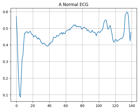
In this example, you will train an autoencoder to detect anomalies on the ECG5000 dataset. This dataset contains 5,000 Electrocardiograms, each with 140 data points. You will use a simplified version of the dataset, where each example has been labeled either 0 (corresponding to an abnormal rhythm), or 1 (corresponding to a normal rhythm). You are interested in identifying the abnormal rhythms.
How will you detect anomalies using an autoencoder? Recall that an autoencoder is trained to minimize reconstruction error. You will train an autoencoder on the normal rhythms only, then use it to reconstruct all the data. Our hypothesis is that the abnormal rhythms will have higher reconstruction error. You will then classify a rhythm as an anomaly if the reconstruction error surpasses a fixed threshold.
Load ECG data
The dataset you will use is based on one from timeseriesclassification.com.
# Download the dataset
dataframe = pd.read_csv('http://storage.googleapis.com/download.tensorflow.org/data/ecg.csv', header=None)
raw_data = dataframe.values
dataframe.head()
# The last element contains the labels
labels = raw_data[:, -1]

# The other data points are the electrocadriogram data
data = raw_data[:, 0:-1]

train_data, test_data, train_labels, test_labels = train_test_split(
    data, labels, test_size=0.2, random_state=21
)
Normalize the data to [0,1].
min_val = tf.reduce_min(train_data)
max_val = tf.reduce_max(train_data)

train_data = (train_data - min_val) / (max_val - min_val)
test_data = (test_data - min_val) / (max_val - min_val)

train_data = tf.cast(train_data, tf.float32)
test_data = tf.cast(test_data, tf.float32)
You will train the autoencoder using only the normal rhythms, which are labeled in this dataset as 1. Separate the normal rhythms from the abnormal rhythms.
train_labels = train_labels.astype(bool)
test_labels = test_labels.astype(bool)

normal_train_data = train_data[train_labels]
normal_test_data = test_data[test_labels]

anomalous_train_data = train_data[~train_labels]
anomalous_test_data = test_data[~test_labels]
Plot a normal ECG.
plt.grid()
plt.plot(np.arange(140), normal_train_data[0])
plt.title("A Normal ECG")
plt.show()
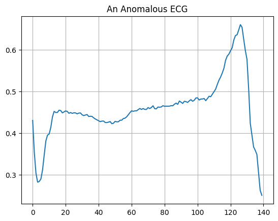
Plot an anomalous ECG.
plt.grid()
plt.plot(np.arange(140), anomalous_train_data[0])
plt.title("An Anomalous ECG")
plt.show()
Build the model
class AnomalyDetector(Model):
  def __init__(self):
    super(AnomalyDetector, self).__init__()
    self.encoder = tf.keras.Sequential([
      layers.Dense(32, activation="relu"),
      layers.Dense(16, activation="relu"),
      layers.Dense(8, activation="relu")])

    self.decoder = tf.keras.Sequential([
      layers.Dense(16, activation="relu"),
      layers.Dense(32, activation="relu"),
      layers.Dense(140, activation="sigmoid")])

  def call(self, x):
    encoded = self.encoder(x)
    decoded = self.decoder(encoded)
    return decoded

autoencoder = AnomalyDetector()
autoencoder.compile(optimizer='adam', loss='mae')
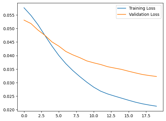
Notice that the autoencoder is trained using only the normal ECGs, but is evaluated using the full test set.
history = autoencoder.fit(normal_train_data, normal_train_data,
          epochs=20,
          batch_size=512,
          validation_data=(test_data, test_data),
          shuffle=True)
Epoch 1/20
5/5 ━━━━━━━━━━━━━━━━━━━━ 5s 551ms/step - loss: 0.0581 - val_loss: 0.0531
Epoch 2/20
5/5 ━━━━━━━━━━━━━━━━━━━━ 0s 13ms/step - loss: 0.0553 - val_loss: 0.0518
Epoch 3/20
5/5 ━━━━━━━━━━━━━━━━━━━━ 0s 13ms/step - loss: 0.0519 - val_loss: 0.0494
Epoch 4/20
5/5 ━━━━━━━━━━━━━━━━━━━━ 0s 13ms/step - loss: 0.0480 - val_loss: 0.0475
Epoch 5/20
5/5 ━━━━━━━━━━━━━━━━━━━━ 0s 13ms/step - loss: 0.0441 - val_loss: 0.0451
Epoch 6/20
5/5 ━━━━━━━━━━━━━━━━━━━━ 0s 13ms/step - loss: 0.0405 - val_loss: 0.0435
Epoch 7/20
5/5 ━━━━━━━━━━━━━━━━━━━━ 0s 13ms/step - loss: 0.0374 - val_loss: 0.0415
Epoch 8/20
5/5 ━━━━━━━━━━━━━━━━━━━━ 0s 13ms/step - loss: 0.0347 - val_loss: 0.0403
Epoch 9/20
5/5 ━━━━━━━━━━━━━━━━━━━━ 0s 13ms/step - loss: 0.0323 - val_loss: 0.0392
Epoch 10/20
5/5 ━━━━━━━━━━━━━━━━━━━━ 0s 13ms/step - loss: 0.0303 - val_loss: 0.0380
Epoch 11/20
5/5 ━━━━━━━━━━━━━━━━━━━━ 0s 13ms/step - loss: 0.0286 - val_loss: 0.0373
Epoch 12/20
5/5 ━━━━━━━━━━━━━━━━━━━━ 0s 13ms/step - loss: 0.0272 - val_loss: 0.0367
Epoch 13/20
5/5 ━━━━━━━━━━━━━━━━━━━━ 0s 13ms/step - loss: 0.0258 - val_loss: 0.0359
Epoch 14/20
5/5 ━━━━━━━━━━━━━━━━━━━━ 0s 13ms/step - loss: 0.0253 - val_loss: 0.0354
Epoch 15/20
5/5 ━━━━━━━━━━━━━━━━━━━━ 0s 13ms/step - loss: 0.0244 - val_loss: 0.0349
Epoch 16/20
5/5 ━━━━━━━━━━━━━━━━━━━━ 0s 13ms/step - loss: 0.0236 - val_loss: 0.0342
Epoch 17/20
5/5 ━━━━━━━━━━━━━━━━━━━━ 0s 13ms/step - loss: 0.0228 - val_loss: 0.0336
Epoch 18/20
5/5 ━━━━━━━━━━━━━━━━━━━━ 0s 13ms/step - loss: 0.0220 - val_loss: 0.0330
Epoch 19/20
5/5 ━━━━━━━━━━━━━━━━━━━━ 0s 13ms/step - loss: 0.0215 - val_loss: 0.0326
Epoch 20/20
5/5 ━━━━━━━━━━━━━━━━━━━━ 0s 13ms/step - loss: 0.0213 - val_loss: 0.0323
plt.plot(history.history["loss"], label="Training Loss")
plt.plot(history.history["val_loss"], label="Validation Loss")
plt.legend()
<matplotlib.legend.Legend at 0x7f8ad34aa730>
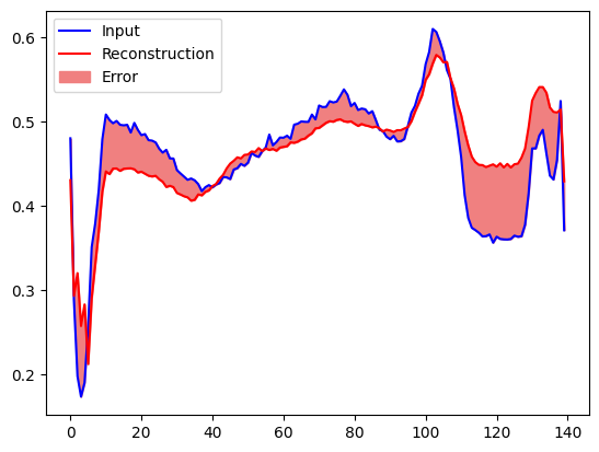
You will soon classify an ECG as anomalous if the reconstruction error is greater than one standard deviation from the normal training examples. First, let's plot a normal ECG from the training set, the reconstruction after it's encoded and decoded by the autoencoder, and the reconstruction error.
encoded_data = autoencoder.encoder(normal_test_data).numpy()
decoded_data = autoencoder.decoder(encoded_data).numpy()

plt.plot(normal_test_data[0], 'b')
plt.plot(decoded_data[0], 'r')
plt.fill_between(np.arange(140), decoded_data[0], normal_test_data[0], color='lightcoral')
plt.legend(labels=["Input", "Reconstruction", "Error"])
plt.show()
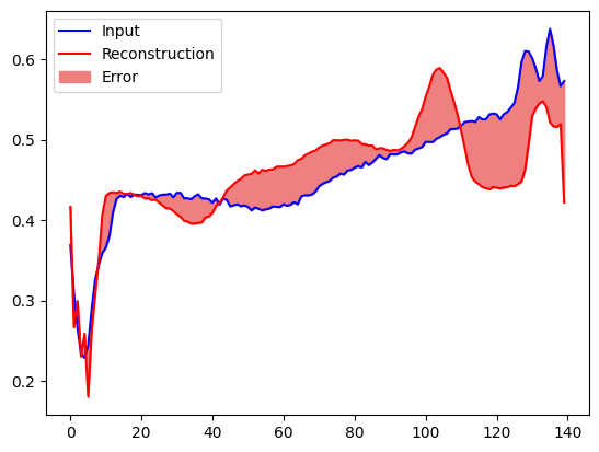
Create a similar plot, this time for an anomalous test example.
encoded_data = autoencoder.encoder(anomalous_test_data).numpy()
decoded_data = autoencoder.decoder(encoded_data).numpy()

plt.plot(anomalous_test_data[0], 'b')
plt.plot(decoded_data[0], 'r')
plt.fill_between(np.arange(140), decoded_data[0], anomalous_test_data[0], color='lightcoral')
plt.legend(labels=["Input", "Reconstruction", "Error"])
plt.show()
Detect anomalies
Detect anomalies by calculating whether the reconstruction loss is greater than a fixed threshold. In this tutorial, you will calculate the mean average error for normal examples from the training set, then classify future examples as anomalous if the reconstruction error is higher than one standard deviation from the training set.
Plot the reconstruction error on normal ECGs from the training set
reconstructions = autoencoder.predict(normal_train_data)
train_loss = tf.keras.losses.mae(reconstructions, normal_train_data)

plt.hist(train_loss[None,:], bins=50)
plt.xlabel("Train loss")
plt.ylabel("No of examples")
plt.show()
74/74 ━━━━━━━━━━━━━━━━━━━━ 1s 6ms/step
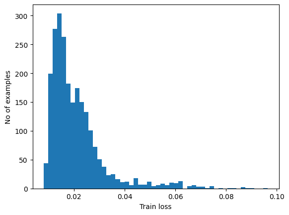
Choose a threshold value that is one standard deviations above the mean.
threshold = np.mean(train_loss) + np.std(train_loss)
print("Threshold: ", threshold)
Threshold: 0.032343477
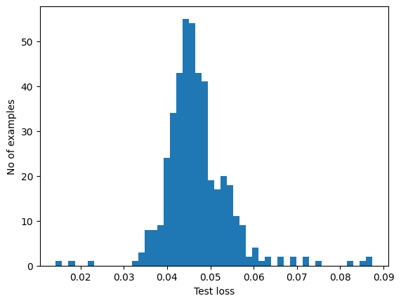
If you examine the reconstruction error for the anomalous examples in the test set, you'll notice most have greater reconstruction error than the threshold. By varing the threshold, you can adjust the precision and recall of your classifier.
reconstructions = autoencoder.predict(anomalous_test_data)
test_loss = tf.keras.losses.mae(reconstructions, anomalous_test_data)

plt.hist(test_loss[None, :], bins=50)
plt.xlabel("Test loss")
plt.ylabel("No of examples")
plt.show()
14/14 ━━━━━━━━━━━━━━━━━━━━ 0s 19ms/step
Classify an ECG as an anomaly if the reconstruction error is greater than the threshold.
def predict(model, data, threshold):
  reconstructions = model(data)
  loss = tf.keras.losses.mae(reconstructions, data)
  return tf.math.less(loss, threshold)

def print_stats(predictions, labels):
  print("Accuracy = {}".format(accuracy_score(labels, predictions)))
  print("Precision = {}".format(precision_score(labels, predictions)))
  print("Recall = {}".format(recall_score(labels, predictions)))
preds = predict(autoencoder, test_data, threshold)
print_stats(preds, test_labels)
Accuracy = 0.944
Precision = 0.9921875
Recall = 0.9071428571428571
Next steps
To learn more about anomaly detection with autoencoders, check out this excellent interactive example built with TensorFlow.js by Victor Dibia. For a real-world use case, you can learn how Airbus Detects Anomalies in ISS Telemetry Data using TensorFlow. To learn more about the basics, consider reading this blog post by François Chollet. For more details, check out chapter 14 from Deep Learning by Ian Goodfellow, Yoshua Bengio, and Aaron Courville.