
|
|
|
 View source on GitHub
|
|
This notebook demonstrates how to train a Variational Autoencoder (VAE) (1, 2) on the MNIST dataset. A VAE is a probabilistic take on the autoencoder, a model which takes high dimensional input data and compresses it into a smaller representation. Unlike a traditional autoencoder, which maps the input onto a latent vector, a VAE maps the input data into the parameters of a probability distribution, such as the mean and variance of a Gaussian. This approach produces a continuous, structured latent space, which is useful for image generation.
Setup
pip install tensorflow-probability# to generate gifspip install imageiopip install git+https://github.com/tensorflow/docs
from IPython import display

import glob
import imageio
import matplotlib.pyplot as plt
import numpy as np
import PIL
import tensorflow as tf
import tensorflow_probability as tfp
import time
2024-08-16 06:55:40.936586: E external/local_xla/xla/stream_executor/cuda/cuda_fft.cc:485] Unable to register cuFFT factory: Attempting to register factory for plugin cuFFT when one has already been registered
2024-08-16 06:55:40.960527: E external/local_xla/xla/stream_executor/cuda/cuda_dnn.cc:8454] Unable to register cuDNN factory: Attempting to register factory for plugin cuDNN when one has already been registered
2024-08-16 06:55:40.967800: E external/local_xla/xla/stream_executor/cuda/cuda_blas.cc:1452] Unable to register cuBLAS factory: Attempting to register factory for plugin cuBLAS when one has already been registered
Load the MNIST dataset
Each MNIST image is originally a vector of 784 integers, each of which is between 0-255 and represents the intensity of a pixel. Model each pixel with a Bernoulli distribution in our model, and statically binarize the dataset.
(train_images, _), (test_images, _) = tf.keras.datasets.mnist.load_data()
def preprocess_images(images):
  images = images.reshape((images.shape[0], 28, 28, 1)) / 255.
  return np.where(images > .5, 1.0, 0.0).astype('float32')

train_images = preprocess_images(train_images)
test_images = preprocess_images(test_images)
train_size = 60000
batch_size = 32
test_size = 10000
Use tf.data to batch and shuffle the data
train_dataset = (tf.data.Dataset.from_tensor_slices(train_images)
                 .shuffle(train_size).batch(batch_size))
test_dataset = (tf.data.Dataset.from_tensor_slices(test_images)
                .shuffle(test_size).batch(batch_size))
WARNING: All log messages before absl::InitializeLog() is called are written to STDERR
I0000 00:00:1723791344.889848  186646 cuda_executor.cc:1015] successful NUMA node read from SysFS had negative value (-1), but there must be at least one NUMA node, so returning NUMA node zero. See more at https://github.com/torvalds/linux/blob/v6.0/Documentation/ABI/testing/sysfs-bus-pci#L344-L355
I0000 00:00:1723791344.893753  186646 cuda_executor.cc:1015] successful NUMA node read from SysFS had negative value (-1), but there must be at least one NUMA node, so returning NUMA node zero. See more at https://github.com/torvalds/linux/blob/v6.0/Documentation/ABI/testing/sysfs-bus-pci#L344-L355
I0000 00:00:1723791344.897409  186646 cuda_executor.cc:1015] successful NUMA node read from SysFS had negative value (-1), but there must be at least one NUMA node, so returning NUMA node zero. See more at https://github.com/torvalds/linux/blob/v6.0/Documentation/ABI/testing/sysfs-bus-pci#L344-L355
I0000 00:00:1723791344.901191  186646 cuda_executor.cc:1015] successful NUMA node read from SysFS had negative value (-1), but there must be at least one NUMA node, so returning NUMA node zero. See more at https://github.com/torvalds/linux/blob/v6.0/Documentation/ABI/testing/sysfs-bus-pci#L344-L355
I0000 00:00:1723791344.913006  186646 cuda_executor.cc:1015] successful NUMA node read from SysFS had negative value (-1), but there must be at least one NUMA node, so returning NUMA node zero. See more at https://github.com/torvalds/linux/blob/v6.0/Documentation/ABI/testing/sysfs-bus-pci#L344-L355
I0000 00:00:1723791344.916554  186646 cuda_executor.cc:1015] successful NUMA node read from SysFS had negative value (-1), but there must be at least one NUMA node, so returning NUMA node zero. See more at https://github.com/torvalds/linux/blob/v6.0/Documentation/ABI/testing/sysfs-bus-pci#L344-L355
I0000 00:00:1723791344.920055  186646 cuda_executor.cc:1015] successful NUMA node read from SysFS had negative value (-1), but there must be at least one NUMA node, so returning NUMA node zero. See more at https://github.com/torvalds/linux/blob/v6.0/Documentation/ABI/testing/sysfs-bus-pci#L344-L355
I0000 00:00:1723791344.923591  186646 cuda_executor.cc:1015] successful NUMA node read from SysFS had negative value (-1), but there must be at least one NUMA node, so returning NUMA node zero. See more at https://github.com/torvalds/linux/blob/v6.0/Documentation/ABI/testing/sysfs-bus-pci#L344-L355
I0000 00:00:1723791344.927078  186646 cuda_executor.cc:1015] successful NUMA node read from SysFS had negative value (-1), but there must be at least one NUMA node, so returning NUMA node zero. See more at https://github.com/torvalds/linux/blob/v6.0/Documentation/ABI/testing/sysfs-bus-pci#L344-L355
I0000 00:00:1723791344.930519  186646 cuda_executor.cc:1015] successful NUMA node read from SysFS had negative value (-1), but there must be at least one NUMA node, so returning NUMA node zero. See more at https://github.com/torvalds/linux/blob/v6.0/Documentation/ABI/testing/sysfs-bus-pci#L344-L355
I0000 00:00:1723791344.933863  186646 cuda_executor.cc:1015] successful NUMA node read from SysFS had negative value (-1), but there must be at least one NUMA node, so returning NUMA node zero. See more at https://github.com/torvalds/linux/blob/v6.0/Documentation/ABI/testing/sysfs-bus-pci#L344-L355
I0000 00:00:1723791344.937424  186646 cuda_executor.cc:1015] successful NUMA node read from SysFS had negative value (-1), but there must be at least one NUMA node, so returning NUMA node zero. See more at https://github.com/torvalds/linux/blob/v6.0/Documentation/ABI/testing/sysfs-bus-pci#L344-L355
I0000 00:00:1723791346.163311  186646 cuda_executor.cc:1015] successful NUMA node read from SysFS had negative value (-1), but there must be at least one NUMA node, so returning NUMA node zero. See more at https://github.com/torvalds/linux/blob/v6.0/Documentation/ABI/testing/sysfs-bus-pci#L344-L355
I0000 00:00:1723791346.165432  186646 cuda_executor.cc:1015] successful NUMA node read from SysFS had negative value (-1), but there must be at least one NUMA node, so returning NUMA node zero. See more at https://github.com/torvalds/linux/blob/v6.0/Documentation/ABI/testing/sysfs-bus-pci#L344-L355
I0000 00:00:1723791346.167444  186646 cuda_executor.cc:1015] successful NUMA node read from SysFS had negative value (-1), but there must be at least one NUMA node, so returning NUMA node zero. See more at https://github.com/torvalds/linux/blob/v6.0/Documentation/ABI/testing/sysfs-bus-pci#L344-L355
I0000 00:00:1723791346.169530  186646 cuda_executor.cc:1015] successful NUMA node read from SysFS had negative value (-1), but there must be at least one NUMA node, so returning NUMA node zero. See more at https://github.com/torvalds/linux/blob/v6.0/Documentation/ABI/testing/sysfs-bus-pci#L344-L355
I0000 00:00:1723791346.171510  186646 cuda_executor.cc:1015] successful NUMA node read from SysFS had negative value (-1), but there must be at least one NUMA node, so returning NUMA node zero. See more at https://github.com/torvalds/linux/blob/v6.0/Documentation/ABI/testing/sysfs-bus-pci#L344-L355
I0000 00:00:1723791346.173466  186646 cuda_executor.cc:1015] successful NUMA node read from SysFS had negative value (-1), but there must be at least one NUMA node, so returning NUMA node zero. See more at https://github.com/torvalds/linux/blob/v6.0/Documentation/ABI/testing/sysfs-bus-pci#L344-L355
I0000 00:00:1723791346.175373  186646 cuda_executor.cc:1015] successful NUMA node read from SysFS had negative value (-1), but there must be at least one NUMA node, so returning NUMA node zero. See more at https://github.com/torvalds/linux/blob/v6.0/Documentation/ABI/testing/sysfs-bus-pci#L344-L355
I0000 00:00:1723791346.177379  186646 cuda_executor.cc:1015] successful NUMA node read from SysFS had negative value (-1), but there must be at least one NUMA node, so returning NUMA node zero. See more at https://github.com/torvalds/linux/blob/v6.0/Documentation/ABI/testing/sysfs-bus-pci#L344-L355
I0000 00:00:1723791346.179286  186646 cuda_executor.cc:1015] successful NUMA node read from SysFS had negative value (-1), but there must be at least one NUMA node, so returning NUMA node zero. See more at https://github.com/torvalds/linux/blob/v6.0/Documentation/ABI/testing/sysfs-bus-pci#L344-L355
I0000 00:00:1723791346.181246  186646 cuda_executor.cc:1015] successful NUMA node read from SysFS had negative value (-1), but there must be at least one NUMA node, so returning NUMA node zero. See more at https://github.com/torvalds/linux/blob/v6.0/Documentation/ABI/testing/sysfs-bus-pci#L344-L355
I0000 00:00:1723791346.183147  186646 cuda_executor.cc:1015] successful NUMA node read from SysFS had negative value (-1), but there must be at least one NUMA node, so returning NUMA node zero. See more at https://github.com/torvalds/linux/blob/v6.0/Documentation/ABI/testing/sysfs-bus-pci#L344-L355
I0000 00:00:1723791346.185151  186646 cuda_executor.cc:1015] successful NUMA node read from SysFS had negative value (-1), but there must be at least one NUMA node, so returning NUMA node zero. See more at https://github.com/torvalds/linux/blob/v6.0/Documentation/ABI/testing/sysfs-bus-pci#L344-L355
I0000 00:00:1723791346.223572  186646 cuda_executor.cc:1015] successful NUMA node read from SysFS had negative value (-1), but there must be at least one NUMA node, so returning NUMA node zero. See more at https://github.com/torvalds/linux/blob/v6.0/Documentation/ABI/testing/sysfs-bus-pci#L344-L355
I0000 00:00:1723791346.225703  186646 cuda_executor.cc:1015] successful NUMA node read from SysFS had negative value (-1), but there must be at least one NUMA node, so returning NUMA node zero. See more at https://github.com/torvalds/linux/blob/v6.0/Documentation/ABI/testing/sysfs-bus-pci#L344-L355
I0000 00:00:1723791346.227658  186646 cuda_executor.cc:1015] successful NUMA node read from SysFS had negative value (-1), but there must be at least one NUMA node, so returning NUMA node zero. See more at https://github.com/torvalds/linux/blob/v6.0/Documentation/ABI/testing/sysfs-bus-pci#L344-L355
I0000 00:00:1723791346.229689  186646 cuda_executor.cc:1015] successful NUMA node read from SysFS had negative value (-1), but there must be at least one NUMA node, so returning NUMA node zero. See more at https://github.com/torvalds/linux/blob/v6.0/Documentation/ABI/testing/sysfs-bus-pci#L344-L355
I0000 00:00:1723791346.231647  186646 cuda_executor.cc:1015] successful NUMA node read from SysFS had negative value (-1), but there must be at least one NUMA node, so returning NUMA node zero. See more at https://github.com/torvalds/linux/blob/v6.0/Documentation/ABI/testing/sysfs-bus-pci#L344-L355
I0000 00:00:1723791346.233622  186646 cuda_executor.cc:1015] successful NUMA node read from SysFS had negative value (-1), but there must be at least one NUMA node, so returning NUMA node zero. See more at https://github.com/torvalds/linux/blob/v6.0/Documentation/ABI/testing/sysfs-bus-pci#L344-L355
I0000 00:00:1723791346.235530  186646 cuda_executor.cc:1015] successful NUMA node read from SysFS had negative value (-1), but there must be at least one NUMA node, so returning NUMA node zero. See more at https://github.com/torvalds/linux/blob/v6.0/Documentation/ABI/testing/sysfs-bus-pci#L344-L355
I0000 00:00:1723791346.237525  186646 cuda_executor.cc:1015] successful NUMA node read from SysFS had negative value (-1), but there must be at least one NUMA node, so returning NUMA node zero. See more at https://github.com/torvalds/linux/blob/v6.0/Documentation/ABI/testing/sysfs-bus-pci#L344-L355
I0000 00:00:1723791346.239502  186646 cuda_executor.cc:1015] successful NUMA node read from SysFS had negative value (-1), but there must be at least one NUMA node, so returning NUMA node zero. See more at https://github.com/torvalds/linux/blob/v6.0/Documentation/ABI/testing/sysfs-bus-pci#L344-L355
I0000 00:00:1723791346.241931  186646 cuda_executor.cc:1015] successful NUMA node read from SysFS had negative value (-1), but there must be at least one NUMA node, so returning NUMA node zero. See more at https://github.com/torvalds/linux/blob/v6.0/Documentation/ABI/testing/sysfs-bus-pci#L344-L355
I0000 00:00:1723791346.244282  186646 cuda_executor.cc:1015] successful NUMA node read from SysFS had negative value (-1), but there must be at least one NUMA node, so returning NUMA node zero. See more at https://github.com/torvalds/linux/blob/v6.0/Documentation/ABI/testing/sysfs-bus-pci#L344-L355
I0000 00:00:1723791346.246700  186646 cuda_executor.cc:1015] successful NUMA node read from SysFS had negative value (-1), but there must be at least one NUMA node, so returning NUMA node zero. See more at https://github.com/torvalds/linux/blob/v6.0/Documentation/ABI/testing/sysfs-bus-pci#L344-L355
Define the encoder and decoder networks with tf.keras.Sequential
In this VAE example, use two small ConvNets for the encoder and decoder networks. In the literature, these networks are also referred to as inference/recognition and generative models respectively. Use tf.keras.Sequential to simplify implementation. Let \(x\) and \(z\) denote the observation and latent variable respectively in the following descriptions.
Encoder network
This defines the approximate posterior distribution \(q(z|x)\), which takes as input an observation and outputs a set of parameters for specifying the conditional distribution of the latent representation \(z\). In this example, simply model the distribution as a diagonal Gaussian, and the network outputs the mean and log-variance parameters of a factorized Gaussian. Output log-variance instead of the variance directly for numerical stability.
Decoder network
This defines the conditional distribution of the observation \(p(x|z)\), which takes a latent sample \(z\) as input and outputs the parameters for a conditional distribution of the observation. Model the latent distribution prior \(p(z)\) as a unit Gaussian.
Reparameterization trick
To generate a sample \(z\) for the decoder during training, you can sample from the latent distribution defined by the parameters outputted by the encoder, given an input observation \(x\). However, this sampling operation creates a bottleneck because backpropagation cannot flow through a random node.
To address this, use a reparameterization trick. In our example, you approximate \(z\) using the decoder parameters and another parameter \(\epsilon\) as follows:
\[z = \mu + \sigma \odot \epsilon\]
where \(\mu\) and \(\sigma\) represent the mean and standard deviation of a Gaussian distribution respectively. They can be derived from the decoder output. The \(\epsilon\) can be thought of as a random noise used to maintain stochasticity of \(z\). Generate \(\epsilon\) from a standard normal distribution.
The latent variable \(z\) is now generated by a function of \(\mu\), \(\sigma\) and \(\epsilon\), which would enable the model to backpropagate gradients in the encoder through \(\mu\) and \(\sigma\) respectively, while maintaining stochasticity through \(\epsilon\).
Network architecture
For the encoder network, use two convolutional layers followed by a fully-connected layer. In the decoder network, mirror this architecture by using a fully-connected layer followed by three convolution transpose layers (a.k.a. deconvolutional layers in some contexts). Note, it's common practice to avoid using batch normalization when training VAEs, since the additional stochasticity due to using mini-batches may aggravate instability on top of the stochasticity from sampling.
class CVAE(tf.keras.Model):
  """Convolutional variational autoencoder."""

  def __init__(self, latent_dim):
    super(CVAE, self).__init__()
    self.latent_dim = latent_dim
    self.encoder = tf.keras.Sequential(
        [
            tf.keras.layers.InputLayer(input_shape=(28, 28, 1)),
            tf.keras.layers.Conv2D(
                filters=32, kernel_size=3, strides=(2, 2), activation='relu'),
            tf.keras.layers.Conv2D(
                filters=64, kernel_size=3, strides=(2, 2), activation='relu'),
            tf.keras.layers.Flatten(),
            # No activation
            tf.keras.layers.Dense(latent_dim + latent_dim),
        ]
    )

    self.decoder = tf.keras.Sequential(
        [
            tf.keras.layers.InputLayer(input_shape=(latent_dim,)),
            tf.keras.layers.Dense(units=7*7*32, activation=tf.nn.relu),
            tf.keras.layers.Reshape(target_shape=(7, 7, 32)),
            tf.keras.layers.Conv2DTranspose(
                filters=64, kernel_size=3, strides=2, padding='same',
                activation='relu'),
            tf.keras.layers.Conv2DTranspose(
                filters=32, kernel_size=3, strides=2, padding='same',
                activation='relu'),
            # No activation
            tf.keras.layers.Conv2DTranspose(
                filters=1, kernel_size=3, strides=1, padding='same'),
        ]
    )

  @tf.function
  def sample(self, eps=None):
    if eps is None:
      eps = tf.random.normal(shape=(100, self.latent_dim))
    return self.decode(eps, apply_sigmoid=True)

  def encode(self, x):
    mean, logvar = tf.split(self.encoder(x), num_or_size_splits=2, axis=1)
    return mean, logvar

  def reparameterize(self, mean, logvar):
    eps = tf.random.normal(shape=mean.shape)
    return eps * tf.exp(logvar * .5) + mean

  def decode(self, z, apply_sigmoid=False):
    logits = self.decoder(z)
    if apply_sigmoid:
      probs = tf.sigmoid(logits)
      return probs
    return logits
Define the loss function and the optimizer
VAEs train by maximizing the evidence lower bound (ELBO) on the marginal log-likelihood:
\[\log p(x) \ge \text{ELBO} = \mathbb{E}_{q(z|x)}\left[\log \frac{p(x, z)}{q(z|x)}\right].\]
In practice, optimize the single sample Monte Carlo estimate of this expectation:
\[\log p(x| z) + \log p(z) - \log q(z|x),\]
where \(z\) is sampled from \(q(z|x)\).
optimizer = tf.keras.optimizers.Adam(1e-4)


def log_normal_pdf(sample, mean, logvar, raxis=1):
  log2pi = tf.math.log(2. * np.pi)
  return tf.reduce_sum(
      -.5 * ((sample - mean) ** 2. * tf.exp(-logvar) + logvar + log2pi),
      axis=raxis)


def compute_loss(model, x):
  mean, logvar = model.encode(x)
  z = model.reparameterize(mean, logvar)
  x_logit = model.decode(z)
  cross_ent = tf.nn.sigmoid_cross_entropy_with_logits(logits=x_logit, labels=x)
  logpx_z = -tf.reduce_sum(cross_ent, axis=[1, 2, 3])
  logpz = log_normal_pdf(z, 0., 0.)
  logqz_x = log_normal_pdf(z, mean, logvar)
  return -tf.reduce_mean(logpx_z + logpz - logqz_x)


@tf.function
def train_step(model, x, optimizer):
  """Executes one training step and returns the loss.

  This function computes the loss and gradients, and uses the latter to
  update the model's parameters.
  """
  with tf.GradientTape() as tape:
    loss = compute_loss(model, x)
  gradients = tape.gradient(loss, model.trainable_variables)
  optimizer.apply_gradients(zip(gradients, model.trainable_variables))
Training
- Start by iterating over the dataset
- During each iteration, pass the image to the encoder to obtain a set of mean and log-variance parameters of the approximate posterior \(q(z|x)\)
- then apply the reparameterization trick to sample from \(q(z|x)\)
- Finally, pass the reparameterized samples to the decoder to obtain the logits of the generative distribution \(p(x|z)\)
- Note: Since you use the dataset loaded by keras with 60k datapoints in the training set and 10k datapoints in the test set, our resulting ELBO on the test set is slightly higher than reported results in the literature which uses dynamic binarization of Larochelle's MNIST.
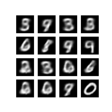
Generating images
- After training, it is time to generate some images
- Start by sampling a set of latent vectors from the unit Gaussian prior distribution \(p(z)\)
- The generator will then convert the latent sample \(z\) to logits of the observation, giving a distribution \(p(x|z)\)
- Here, plot the probabilities of Bernoulli distributions
epochs = 10
# set the dimensionality of the latent space to a plane for visualization later
latent_dim = 2
num_examples_to_generate = 16

# keeping the random vector constant for generation (prediction) so
# it will be easier to see the improvement.
random_vector_for_generation = tf.random.normal(
    shape=[num_examples_to_generate, latent_dim])
model = CVAE(latent_dim)
/tmpfs/src/tf_docs_env/lib/python3.9/site-packages/keras/src/layers/core/input_layer.py:26: UserWarning: Argument `input_shape` is deprecated. Use `shape` instead.
  warnings.warn(
def generate_and_save_images(model, epoch, test_sample):
  mean, logvar = model.encode(test_sample)
  z = model.reparameterize(mean, logvar)
  predictions = model.sample(z)
  fig = plt.figure(figsize=(4, 4))

  for i in range(predictions.shape[0]):
    plt.subplot(4, 4, i + 1)
    plt.imshow(predictions[i, :, :, 0], cmap='gray')
    plt.axis('off')

  # tight_layout minimizes the overlap between 2 sub-plots
  plt.savefig('image_at_epoch_{:04d}.png'.format(epoch))
  plt.show()
# Pick a sample of the test set for generating output images
assert batch_size >= num_examples_to_generate
for test_batch in test_dataset.take(1):
  test_sample = test_batch[0:num_examples_to_generate, :, :, :]
generate_and_save_images(model, 0, test_sample)

for epoch in range(1, epochs + 1):
  start_time = time.time()
  for train_x in train_dataset:
    train_step(model, train_x, optimizer)
  end_time = time.time()

  loss = tf.keras.metrics.Mean()
  for test_x in test_dataset:
    loss(compute_loss(model, test_x))
  elbo = -loss.result()
  display.clear_output(wait=False)
  print('Epoch: {}, Test set ELBO: {}, time elapse for current epoch: {}'
        .format(epoch, elbo, end_time - start_time))
  generate_and_save_images(model, epoch, test_sample)
Epoch: 10, Test set ELBO: -156.98243713378906, time elapse for current epoch: 7.436727523803711
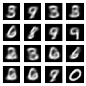
Display a generated image from the last training epoch
def display_image(epoch_no):
  return PIL.Image.open('image_at_epoch_{:04d}.png'.format(epoch_no))
plt.imshow(display_image(epoch))
plt.axis('off')  # Display images
(-0.5, 399.5, 399.5, -0.5)
Display an animated GIF of all the saved images
anim_file = 'cvae.gif'

with imageio.get_writer(anim_file, mode='I') as writer:
  filenames = glob.glob('image*.png')
  filenames = sorted(filenames)
  for filename in filenames:
    image = imageio.imread(filename)
    writer.append_data(image)
  image = imageio.imread(filename)
  writer.append_data(image)
/tmpfs/tmp/ipykernel_186646/1290275450.py:7: DeprecationWarning: Starting with ImageIO v3 the behavior of this function will switch to that of iio.v3.imread. To keep the current behavior (and make this warning disappear) use `import imageio.v2 as imageio` or call `imageio.v2.imread` directly.
  image = imageio.imread(filename)
/tmpfs/tmp/ipykernel_186646/1290275450.py:9: DeprecationWarning: Starting with ImageIO v3 the behavior of this function will switch to that of iio.v3.imread. To keep the current behavior (and make this warning disappear) use `import imageio.v2 as imageio` or call `imageio.v2.imread` directly.
  image = imageio.imread(filename)
import tensorflow_docs.vis.embed as embed
embed.embed_file(anim_file)
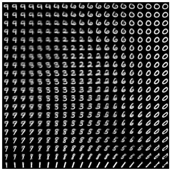
Display a 2D manifold of digits from the latent space
Running the code below will show a continuous distribution of the different digit classes, with each digit morphing into another across the 2D latent space. Use TensorFlow Probability to generate a standard normal distribution for the latent space.
def plot_latent_images(model, n, digit_size=28):
  """Plots n x n digit images decoded from the latent space."""

  norm = tfp.distributions.Normal(0, 1)
  grid_x = norm.quantile(np.linspace(0.05, 0.95, n))
  grid_y = norm.quantile(np.linspace(0.05, 0.95, n))
  image_width = digit_size*n
  image_height = image_width
  image = np.zeros((image_height, image_width))

  for i, yi in enumerate(grid_x):
    for j, xi in enumerate(grid_y):
      z = np.array([[xi, yi]])
      x_decoded = model.sample(z)
      digit = tf.reshape(x_decoded[0], (digit_size, digit_size))
      image[i * digit_size: (i + 1) * digit_size,
            j * digit_size: (j + 1) * digit_size] = digit.numpy()

  plt.figure(figsize=(10, 10))
  plt.imshow(image, cmap='Greys_r')
  plt.axis('Off')
  plt.show()
plot_latent_images(model, 20)
W0000 00:00:1723791474.856095  186849 gpu_timer.cc:114] Skipping the delay kernel, measurement accuracy will be reduced
W0000 00:00:1723791474.857363  186849 gpu_timer.cc:114] Skipping the delay kernel, measurement accuracy will be reduced
W0000 00:00:1723791474.858508  186849 gpu_timer.cc:114] Skipping the delay kernel, measurement accuracy will be reduced
W0000 00:00:1723791474.859625  186849 gpu_timer.cc:114] Skipping the delay kernel, measurement accuracy will be reduced
W0000 00:00:1723791474.860753  186849 gpu_timer.cc:114] Skipping the delay kernel, measurement accuracy will be reduced
W0000 00:00:1723791474.862036  186849 gpu_timer.cc:114] Skipping the delay kernel, measurement accuracy will be reduced
W0000 00:00:1723791474.863389  186849 gpu_timer.cc:114] Skipping the delay kernel, measurement accuracy will be reduced
W0000 00:00:1723791474.869764  186849 gpu_timer.cc:114] Skipping the delay kernel, measurement accuracy will be reduced
W0000 00:00:1723791474.872697  186849 gpu_timer.cc:114] Skipping the delay kernel, measurement accuracy will be reduced
W0000 00:00:1723791474.873874  186849 gpu_timer.cc:114] Skipping the delay kernel, measurement accuracy will be reduced
W0000 00:00:1723791474.875030  186849 gpu_timer.cc:114] Skipping the delay kernel, measurement accuracy will be reduced
W0000 00:00:1723791474.876195  186849 gpu_timer.cc:114] Skipping the delay kernel, measurement accuracy will be reduced
W0000 00:00:1723791474.877401  186849 gpu_timer.cc:114] Skipping the delay kernel, measurement accuracy will be reduced
W0000 00:00:1723791474.878686  186849 gpu_timer.cc:114] Skipping the delay kernel, measurement accuracy will be reduced
W0000 00:00:1723791474.880003  186849 gpu_timer.cc:114] Skipping the delay kernel, measurement accuracy will be reduced
W0000 00:00:1723791474.881685  186849 gpu_timer.cc:114] Skipping the delay kernel, measurement accuracy will be reduced
W0000 00:00:1723791474.885242  186849 gpu_timer.cc:114] Skipping the delay kernel, measurement accuracy will be reduced
W0000 00:00:1723791474.886407  186849 gpu_timer.cc:114] Skipping the delay kernel, measurement accuracy will be reduced
W0000 00:00:1723791474.887527  186849 gpu_timer.cc:114] Skipping the delay kernel, measurement accuracy will be reduced
W0000 00:00:1723791474.888669  186849 gpu_timer.cc:114] Skipping the delay kernel, measurement accuracy will be reduced
W0000 00:00:1723791474.889868  186849 gpu_timer.cc:114] Skipping the delay kernel, measurement accuracy will be reduced
W0000 00:00:1723791474.891009  186849 gpu_timer.cc:114] Skipping the delay kernel, measurement accuracy will be reduced
W0000 00:00:1723791474.892217  186849 gpu_timer.cc:114] Skipping the delay kernel, measurement accuracy will be reduced
W0000 00:00:1723791474.893383  186849 gpu_timer.cc:114] Skipping the delay kernel, measurement accuracy will be reduced
W0000 00:00:1723791474.894542  186849 gpu_timer.cc:114] Skipping the delay kernel, measurement accuracy will be reduced
W0000 00:00:1723791474.895693  186849 gpu_timer.cc:114] Skipping the delay kernel, measurement accuracy will be reduced

Next steps
This tutorial has demonstrated how to implement a convolutional variational autoencoder using TensorFlow.
As a next step, you could try to improve the model output by increasing the network size.
For instance, you could try setting the filter parameters for each of the Conv2D and Conv2DTranspose layers to 512.
Note that in order to generate the final 2D latent image plot, you would need to keep latent_dim to 2. Also, the training time would increase as the network size increases.
You could also try implementing a VAE using a different dataset, such as CIFAR-10.
VAEs can be implemented in several different styles and of varying complexity. You can find additional implementations in the following sources:
- Variational AutoEncoder (keras.io)
- VAE example from "Writing custom layers and models" guide (tensorflow.org)
- TFP Probabilistic Layers: Variational Auto Encoder
If you'd like to learn more about the details of VAEs, please refer to An Introduction to Variational Autoencoders.