
| | |  GitHub पर स्रोत देखें GitHub पर स्रोत देखें | |
यह नोटबुक सशर्त GAN का उपयोग करके छवि से छवि अनुवाद में अयुग्मित छवि को प्रदर्शित करता है, जैसा कि साइकिल-संगत प्रतिकूल नेटवर्क का उपयोग करते हुए अप्रकाशित छवि-से-छवि अनुवाद में वर्णित है, जिसे CycleGAN भी कहा जाता है। पेपर एक ऐसी विधि का प्रस्ताव करता है जो एक छवि डोमेन की विशेषताओं को कैप्चर कर सकती है और यह पता लगा सकती है कि इन विशेषताओं को किसी अन्य छवि डोमेन में कैसे अनुवादित किया जा सकता है, सभी किसी भी युग्मित प्रशिक्षण उदाहरणों के अभाव में।
यह नोटबुक मानता है कि आप Pix2Pix से परिचित हैं, जिसके बारे में आप Pix2Pix ट्यूटोरियल में सीख सकते हैं। साइकिलगैन के लिए कोड समान है, मुख्य अंतर एक अतिरिक्त नुकसान फ़ंक्शन है, और अप्रकाशित प्रशिक्षण डेटा का उपयोग है।
साइकिलगैन युग्मित डेटा की आवश्यकता के बिना प्रशिक्षण को सक्षम करने के लिए एक चक्र स्थिरता हानि का उपयोग करता है। दूसरे शब्दों में, यह स्रोत और लक्ष्य डोमेन के बीच एक-से-एक मैपिंग के बिना एक डोमेन से दूसरे डोमेन में अनुवाद कर सकता है।
यह फोटो-एन्हांसमेंट, इमेज कलराइजेशन, स्टाइल ट्रांसफर इत्यादि जैसे कई दिलचस्प कार्यों को करने की संभावना को खोलता है। आपको केवल स्रोत और लक्ष्य डेटासेट की आवश्यकता होती है (जो केवल छवियों की निर्देशिका है)।
इनपुट पाइपलाइन सेट करें
tensorflow_examples पैकेज स्थापित करें जो जनरेटर और विवेचक को आयात करने में सक्षम बनाता है।
pip install git+https://github.com/tensorflow/examples.git
import tensorflow as tf
import tensorflow_datasets as tfds
from tensorflow_examples.models.pix2pix import pix2pix

import os
import time
import matplotlib.pyplot as plt
from IPython.display import clear_output

AUTOTUNE = tf.data.AUTOTUNE
इनपुट पाइपलाइन
यह ट्यूटोरियल एक मॉडल को घोड़ों की छवियों से ज़ेबरा की छवियों में अनुवाद करने के लिए प्रशिक्षित करता है। आप इस डेटासेट और इसी तरह के डेटासेट यहां पा सकते हैं।
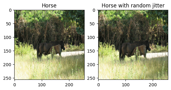
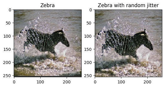
जैसा कि पेपर में उल्लेख किया गया है, प्रशिक्षण डेटासेट में रैंडम जिटरिंग और मिररिंग लागू करें। ये कुछ छवि वृद्धि तकनीकें हैं जो ओवरफिटिंग से बचाती हैं।
यह ठीक वैसा ही है जैसा कि पिक्स2पिक्स में किया गया था
- यादृच्छिक घबराहट में, छवि का आकार बदलकर
286 x 286कर दिया जाता है और फिर यादृच्छिक रूप से256 x 256पर काट दिया जाता है। - यादृच्छिक मिररिंग में, छवि बेतरतीब ढंग से क्षैतिज रूप से फ़्लिप की जाती है अर्थात बाएं से दाएं।
dataset, metadata = tfds.load('cycle_gan/horse2zebra',
                              with_info=True, as_supervised=True)

train_horses, train_zebras = dataset['trainA'], dataset['trainB']
test_horses, test_zebras = dataset['testA'], dataset['testB']
BUFFER_SIZE = 1000
BATCH_SIZE = 1
IMG_WIDTH = 256
IMG_HEIGHT = 256
def random_crop(image):
  cropped_image = tf.image.random_crop(
      image, size=[IMG_HEIGHT, IMG_WIDTH, 3])

  return cropped_image
# normalizing the images to [-1, 1]
def normalize(image):
  image = tf.cast(image, tf.float32)
  image = (image / 127.5) - 1
  return image
def random_jitter(image):
  # resizing to 286 x 286 x 3
  image = tf.image.resize(image, [286, 286],
                          method=tf.image.ResizeMethod.NEAREST_NEIGHBOR)

  # randomly cropping to 256 x 256 x 3
  image = random_crop(image)

  # random mirroring
  image = tf.image.random_flip_left_right(image)

  return image
def preprocess_image_train(image, label):
  image = random_jitter(image)
  image = normalize(image)
  return image
def preprocess_image_test(image, label):
  image = normalize(image)
  return image
train_horses = train_horses.cache().map(
    preprocess_image_train, num_parallel_calls=AUTOTUNE).shuffle(
    BUFFER_SIZE).batch(BATCH_SIZE)

train_zebras = train_zebras.cache().map(
    preprocess_image_train, num_parallel_calls=AUTOTUNE).shuffle(
    BUFFER_SIZE).batch(BATCH_SIZE)

test_horses = test_horses.map(
    preprocess_image_test, num_parallel_calls=AUTOTUNE).cache().shuffle(
    BUFFER_SIZE).batch(BATCH_SIZE)

test_zebras = test_zebras.map(
    preprocess_image_test, num_parallel_calls=AUTOTUNE).cache().shuffle(
    BUFFER_SIZE).batch(BATCH_SIZE)
sample_horse = next(iter(train_horses))
sample_zebra = next(iter(train_zebras))
plt.subplot(121)
plt.title('Horse')
plt.imshow(sample_horse[0] * 0.5 + 0.5)

plt.subplot(122)
plt.title('Horse with random jitter')
plt.imshow(random_jitter(sample_horse[0]) * 0.5 + 0.5)
2022-01-26 02:38:15.762422: W tensorflow/core/kernels/data/cache_dataset_ops.cc:768] The calling iterator did not fully read the dataset being cached. In order to avoid unexpected truncation of the dataset, the partially cached contents of the dataset  will be discarded. This can happen if you have an input pipeline similar to `dataset.cache().take(k).repeat()`. You should use `dataset.take(k).cache().repeat()` instead.
2022-01-26 02:38:19.927846: W tensorflow/core/kernels/data/cache_dataset_ops.cc:768] The calling iterator did not fully read the dataset being cached. In order to avoid unexpected truncation of the dataset, the partially cached contents of the dataset  will be discarded. This can happen if you have an input pipeline similar to `dataset.cache().take(k).repeat()`. You should use `dataset.take(k).cache().repeat()` instead.
<matplotlib.image.AxesImage at 0x7f7cf83e0050>
plt.subplot(121)
plt.title('Zebra')
plt.imshow(sample_zebra[0] * 0.5 + 0.5)

plt.subplot(122)
plt.title('Zebra with random jitter')
plt.imshow(random_jitter(sample_zebra[0]) * 0.5 + 0.5)
<matplotlib.image.AxesImage at 0x7f7cf8139490>
Pix2Pix मॉडल आयात और पुन: उपयोग करें
स्थापित tensorflow_examples पैकेज के माध्यम से Pix2Pix में उपयोग किए गए जनरेटर और विवेचक को आयात करें।
इस ट्यूटोरियल में उपयोग किया गया मॉडल आर्किटेक्चर बहुत कुछ वैसा ही है जैसा कि pix2pix में उपयोग किया गया था। इनमें से कुछ अंतर हैं:
- साइकिलगन बैच सामान्यीकरण के बजाय उदाहरण सामान्यीकरण का उपयोग करता है।
- साइकिलगैन पेपर एक संशोधित
resnetआधारित जनरेटर का उपयोग करता है। यह ट्यूटोरियल सादगी के लिए एक संशोधितunetजनरेटर का उपयोग कर रहा है।
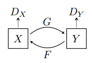
यहां 2 जेनरेटर (जी और एफ) और 2 डिस्क्रिमिनेटर (एक्स और वाई) प्रशिक्षित किए जा रहे हैं।
- जेनरेटर
GइमेजXको इमेजYमें बदलना सीखता है। \((G: X -> Y)\) - जेनरेटर
FइमेजYको इमेजXमें बदलना सीखता है। \((F: Y -> X)\) -
D_XछविXऔर उत्पन्न छविX(F(Y)) के बीच अंतर करना सीखता है। -
D_YछविYऔर उत्पन्न छविY(G(X)) के बीच अंतर करना सीखता है।
OUTPUT_CHANNELS = 3

generator_g = pix2pix.unet_generator(OUTPUT_CHANNELS, norm_type='instancenorm')
generator_f = pix2pix.unet_generator(OUTPUT_CHANNELS, norm_type='instancenorm')

discriminator_x = pix2pix.discriminator(norm_type='instancenorm', target=False)
discriminator_y = pix2pix.discriminator(norm_type='instancenorm', target=False)
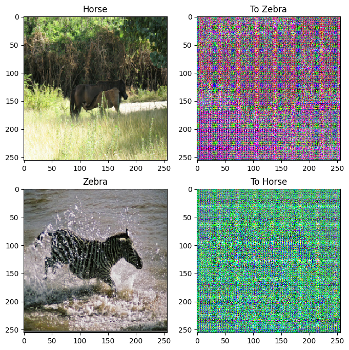
to_zebra = generator_g(sample_horse)
to_horse = generator_f(sample_zebra)
plt.figure(figsize=(8, 8))
contrast = 8

imgs = [sample_horse, to_zebra, sample_zebra, to_horse]
title = ['Horse', 'To Zebra', 'Zebra', 'To Horse']

for i in range(len(imgs)):
  plt.subplot(2, 2, i+1)
  plt.title(title[i])
  if i % 2 == 0:
    plt.imshow(imgs[i][0] * 0.5 + 0.5)
  else:
    plt.imshow(imgs[i][0] * 0.5 * contrast + 0.5)
plt.show()
WARNING:matplotlib.image:Clipping input data to the valid range for imshow with RGB data ([0..1] for floats or [0..255] for integers).
WARNING:matplotlib.image:Clipping input data to the valid range for imshow with RGB data ([0..1] for floats or [0..255] for integers).
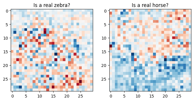
plt.figure(figsize=(8, 8))

plt.subplot(121)
plt.title('Is a real zebra?')
plt.imshow(discriminator_y(sample_zebra)[0, ..., -1], cmap='RdBu_r')

plt.subplot(122)
plt.title('Is a real horse?')
plt.imshow(discriminator_x(sample_horse)[0, ..., -1], cmap='RdBu_r')

plt.show()
हानि कार्य
CycleGAN में, प्रशिक्षित करने के लिए कोई युग्मित डेटा नहीं है, इसलिए इस बात की कोई गारंटी नहीं है कि प्रशिक्षण के दौरान इनपुट x और लक्ष्य y जोड़ी सार्थक हैं। इस प्रकार यह लागू करने के लिए कि नेटवर्क सही मैपिंग सीखता है, लेखक चक्र स्थिरता हानि का प्रस्ताव करते हैं।
विवेचक हानि और जनरेटर हानि pix2pix में उपयोग किए जाने वाले समान हैं।
LAMBDA = 10
loss_obj = tf.keras.losses.BinaryCrossentropy(from_logits=True)
def discriminator_loss(real, generated):
  real_loss = loss_obj(tf.ones_like(real), real)

  generated_loss = loss_obj(tf.zeros_like(generated), generated)

  total_disc_loss = real_loss + generated_loss

  return total_disc_loss * 0.5
def generator_loss(generated):
  return loss_obj(tf.ones_like(generated), generated)
चक्र स्थिरता का मतलब है कि परिणाम मूल इनपुट के करीब होना चाहिए। उदाहरण के लिए, यदि कोई किसी वाक्य का अंग्रेजी से फ्रेंच में अनुवाद करता है, और फिर उसका फ्रेंच से अंग्रेजी में अनुवाद करता है, तो परिणामी वाक्य मूल वाक्य के समान होना चाहिए।
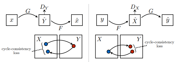
चक्र स्थिरता हानि में,
- छवि \(X\) जनरेटर \(G\) माध्यम से पारित किया जाता है जो उत्पन्न छवि \(\hat{Y}\)उत्पन्न करता है।
- उत्पन्न छवि \(\hat{Y}\) जनरेटर \(F\) माध्यम से पारित किया जाता है जो चक्रीय छवि उत्पन्न करता है \(\hat{X}\)।
- माध्य निरपेक्ष त्रुटि की गणना \(X\) और \(\hat{X}\)के बीच की जाती है।
\[forward\ cycle\ consistency\ loss: X -> G(X) -> F(G(X)) \sim \hat{X}\]
\[backward\ cycle\ consistency\ loss: Y -> F(Y) -> G(F(Y)) \sim \hat{Y}\]
def calc_cycle_loss(real_image, cycled_image):
  loss1 = tf.reduce_mean(tf.abs(real_image - cycled_image))

  return LAMBDA * loss1
जैसा कि ऊपर दिखाया गया है, जनरेटर \(G\) छवि \(X\) को छवि \(Y\)placeholder15 में अनुवाद करने के लिए जिम्मेदार है। आइडेंटिटी लॉस कहता है कि, अगर आपने इमेज \(Y\) 16 को जनरेटर \(G\)प्लेसहोल्डर17 को फीड किया है, तो उसे वास्तविक इमेज \(Y\) या इमेज \(Y\)प्लेसहोल्डर19 के करीब कुछ देना चाहिए।
यदि आप ज़ेबरा-टू-हॉर्स मॉडल को घोड़े पर या हॉर्स-टू-ज़ेबरा मॉडल को ज़ेबरा पर चलाते हैं, तो इसे छवि को अधिक संशोधित नहीं करना चाहिए क्योंकि छवि में पहले से ही लक्ष्य वर्ग है।
\[Identity\ loss = |G(Y) - Y| + |F(X) - X|\]
def identity_loss(real_image, same_image):
  loss = tf.reduce_mean(tf.abs(real_image - same_image))
  return LAMBDA * 0.5 * loss
सभी जनरेटर और विवेचकों के लिए ऑप्टिमाइज़र प्रारंभ करें।
generator_g_optimizer = tf.keras.optimizers.Adam(2e-4, beta_1=0.5)
generator_f_optimizer = tf.keras.optimizers.Adam(2e-4, beta_1=0.5)

discriminator_x_optimizer = tf.keras.optimizers.Adam(2e-4, beta_1=0.5)
discriminator_y_optimizer = tf.keras.optimizers.Adam(2e-4, beta_1=0.5)
चौकियों
checkpoint_path = "./checkpoints/train"

ckpt = tf.train.Checkpoint(generator_g=generator_g,
                           generator_f=generator_f,
                           discriminator_x=discriminator_x,
                           discriminator_y=discriminator_y,
                           generator_g_optimizer=generator_g_optimizer,
                           generator_f_optimizer=generator_f_optimizer,
                           discriminator_x_optimizer=discriminator_x_optimizer,
                           discriminator_y_optimizer=discriminator_y_optimizer)

ckpt_manager = tf.train.CheckpointManager(ckpt, checkpoint_path, max_to_keep=5)

# if a checkpoint exists, restore the latest checkpoint.
if ckpt_manager.latest_checkpoint:
  ckpt.restore(ckpt_manager.latest_checkpoint)
  print ('Latest checkpoint restored!!')
प्रशिक्षण
EPOCHS = 40
def generate_images(model, test_input):
  prediction = model(test_input)

  plt.figure(figsize=(12, 12))

  display_list = [test_input[0], prediction[0]]
  title = ['Input Image', 'Predicted Image']

  for i in range(2):
    plt.subplot(1, 2, i+1)
    plt.title(title[i])
    # getting the pixel values between [0, 1] to plot it.
    plt.imshow(display_list[i] * 0.5 + 0.5)
    plt.axis('off')
  plt.show()
भले ही प्रशिक्षण लूप जटिल लगता है, इसमें चार बुनियादी चरण होते हैं:
- भविष्यवाणियां प्राप्त करें।
- नुकसान की गणना करें।
- बैकप्रोपेगेशन का उपयोग करके ग्रेडिएंट्स की गणना करें।
- ऑप्टिमाइज़र पर ग्रेडिएंट लागू करें।
@tf.function
def train_step(real_x, real_y):
  # persistent is set to True because the tape is used more than
  # once to calculate the gradients.
  with tf.GradientTape(persistent=True) as tape:
    # Generator G translates X -> Y
    # Generator F translates Y -> X.

    fake_y = generator_g(real_x, training=True)
    cycled_x = generator_f(fake_y, training=True)

    fake_x = generator_f(real_y, training=True)
    cycled_y = generator_g(fake_x, training=True)

    # same_x and same_y are used for identity loss.
    same_x = generator_f(real_x, training=True)
    same_y = generator_g(real_y, training=True)

    disc_real_x = discriminator_x(real_x, training=True)
    disc_real_y = discriminator_y(real_y, training=True)

    disc_fake_x = discriminator_x(fake_x, training=True)
    disc_fake_y = discriminator_y(fake_y, training=True)

    # calculate the loss
    gen_g_loss = generator_loss(disc_fake_y)
    gen_f_loss = generator_loss(disc_fake_x)

    total_cycle_loss = calc_cycle_loss(real_x, cycled_x) + calc_cycle_loss(real_y, cycled_y)

    # Total generator loss = adversarial loss + cycle loss
    total_gen_g_loss = gen_g_loss + total_cycle_loss + identity_loss(real_y, same_y)
    total_gen_f_loss = gen_f_loss + total_cycle_loss + identity_loss(real_x, same_x)

    disc_x_loss = discriminator_loss(disc_real_x, disc_fake_x)
    disc_y_loss = discriminator_loss(disc_real_y, disc_fake_y)

  # Calculate the gradients for generator and discriminator
  generator_g_gradients = tape.gradient(total_gen_g_loss,
                                        generator_g.trainable_variables)
  generator_f_gradients = tape.gradient(total_gen_f_loss,
                                        generator_f.trainable_variables)

  discriminator_x_gradients = tape.gradient(disc_x_loss,
                                            discriminator_x.trainable_variables)
  discriminator_y_gradients = tape.gradient(disc_y_loss,
                                            discriminator_y.trainable_variables)

  # Apply the gradients to the optimizer
  generator_g_optimizer.apply_gradients(zip(generator_g_gradients,
                                            generator_g.trainable_variables))

  generator_f_optimizer.apply_gradients(zip(generator_f_gradients,
                                            generator_f.trainable_variables))

  discriminator_x_optimizer.apply_gradients(zip(discriminator_x_gradients,
                                                discriminator_x.trainable_variables))

  discriminator_y_optimizer.apply_gradients(zip(discriminator_y_gradients,
                                                discriminator_y.trainable_variables))
for epoch in range(EPOCHS):
  start = time.time()

  n = 0
  for image_x, image_y in tf.data.Dataset.zip((train_horses, train_zebras)):
    train_step(image_x, image_y)
    if n % 10 == 0:
      print ('.', end='')
    n += 1

  clear_output(wait=True)
  # Using a consistent image (sample_horse) so that the progress of the model
  # is clearly visible.
  generate_images(generator_g, sample_horse)

  if (epoch + 1) % 5 == 0:
    ckpt_save_path = ckpt_manager.save()
    print ('Saving checkpoint for epoch {} at {}'.format(epoch+1,
                                                         ckpt_save_path))

  print ('Time taken for epoch {} is {} sec\n'.format(epoch + 1,
                                                      time.time()-start))
Saving checkpoint for epoch 40 at ./checkpoints/train/ckpt-8
Time taken for epoch 40 is 166.64579939842224 sec
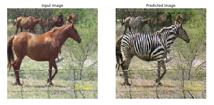
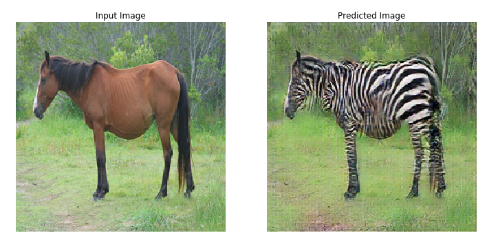
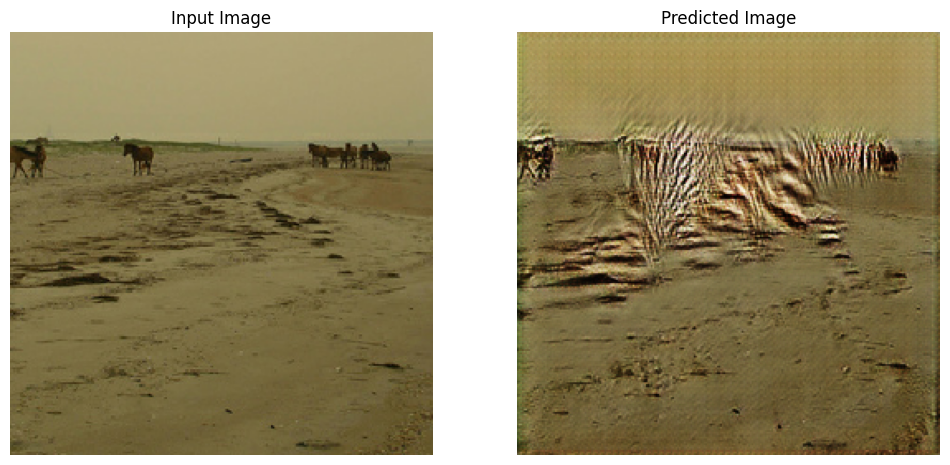
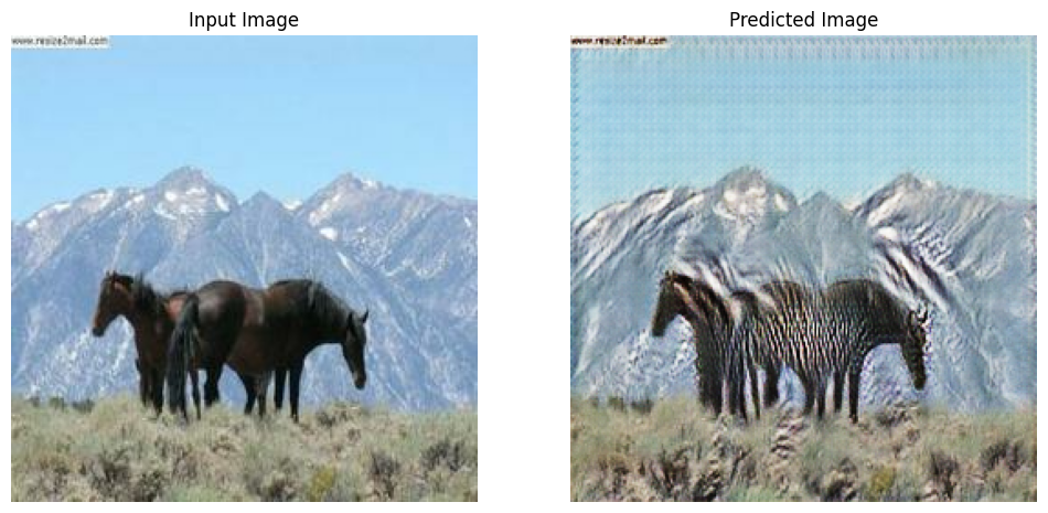
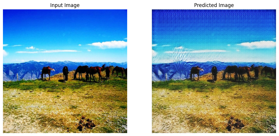
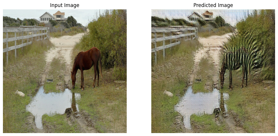
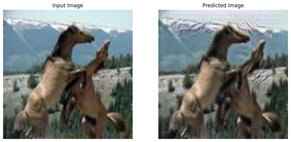
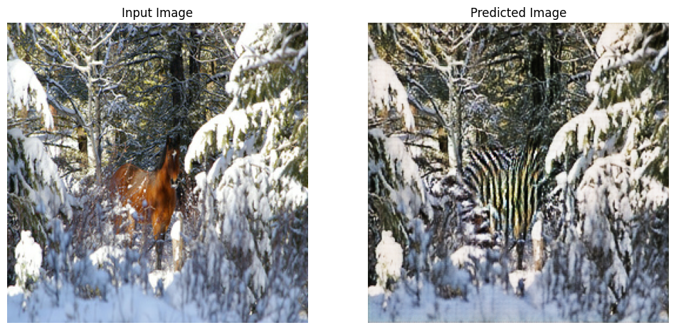
परीक्षण डेटासेट का उपयोग करके उत्पन्न करें
# Run the trained model on the test dataset
for inp in test_horses.take(5):
  generate_images(generator_g, inp)
अगले कदम
इस ट्यूटोरियल में दिखाया गया है कि Pix2Pix ट्यूटोरियल में लागू जनरेटर और डिस्क्रिमिनेटर से साइकिलगैन को कैसे लागू किया जाए। अगले चरण के रूप में, आप TensorFlow Datasets से भिन्न डेटासेट का उपयोग करने का प्रयास कर सकते हैं।
आप परिणामों को बेहतर बनाने के लिए बड़ी संख्या में युगों के लिए प्रशिक्षण भी ले सकते हैं, या आप यहां इस्तेमाल किए गए यू-नेट जनरेटर के बजाय पेपर में उपयोग किए गए संशोधित रेसनेट जनरेटर को लागू कर सकते हैं।