
| | |  GitHub पर स्रोत देखें GitHub पर स्रोत देखें | |
इस ट्यूटोरियल में डीपड्रीम का न्यूनतम कार्यान्वयन शामिल है, जैसा कि अलेक्जेंडर मोर्डविंटसेव द्वारा इस ब्लॉग पोस्ट में वर्णित है।
डीपड्रीम एक ऐसा प्रयोग है जो तंत्रिका नेटवर्क द्वारा सीखे गए पैटर्न की कल्पना करता है। उसी तरह जब कोई बच्चा बादलों को देखता है और यादृच्छिक आकृतियों की व्याख्या करने की कोशिश करता है, डीपड्रीम एक छवि में देखे जाने वाले पैटर्न की अधिक व्याख्या और सुधार करता है।
यह नेटवर्क के माध्यम से एक छवि को अग्रेषित करके ऐसा करता है, फिर किसी विशेष परत की सक्रियता के संबंध में छवि के ढाल की गणना करता है। फिर इन सक्रियणों को बढ़ाने के लिए छवि को संशोधित किया जाता है, नेटवर्क द्वारा देखे जाने वाले पैटर्न को बढ़ाता है, और परिणामस्वरूप एक स्वप्न जैसी छवि बनती है। इस प्रक्रिया को "इंसेप्शनिज्म" ( इंसेप्शननेट का एक संदर्भ, और फिल्म इंसेप्शन) करार दिया गया था।
आइए प्रदर्शित करें कि आप एक तंत्रिका नेटवर्क को "सपना" कैसे बना सकते हैं और एक छवि में देखे जाने वाले असली पैटर्न को बढ़ा सकते हैं।
import tensorflow as tf
import numpy as np

import matplotlib as mpl

import IPython.display as display
import PIL.Image
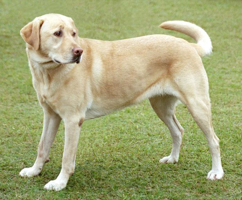
सपने देखने के लिए एक छवि चुनें-आईएफई
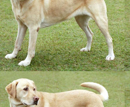
इस ट्यूटोरियल के लिए, आइए लैब्राडोर की छवि का उपयोग करें।
url = 'https://storage.googleapis.com/download.tensorflow.org/example_images/YellowLabradorLooking_new.jpg'
# Download an image and read it into a NumPy array.
def download(url, max_dim=None):
  name = url.split('/')[-1]
  image_path = tf.keras.utils.get_file(name, origin=url)
  img = PIL.Image.open(image_path)
  if max_dim:
    img.thumbnail((max_dim, max_dim))
  return np.array(img)

# Normalize an image
def deprocess(img):
  img = 255*(img + 1.0)/2.0
  return tf.cast(img, tf.uint8)

# Display an image
def show(img):
  display.display(PIL.Image.fromarray(np.array(img)))


# Downsizing the image makes it easier to work with.
original_img = download(url, max_dim=500)
show(original_img)
display.display(display.HTML('Image cc-by: <a "href=https://commons.wikimedia.org/wiki/File:Felis_catus-cat_on_snow.jpg">Von.grzanka</a>'))
सुविधा निष्कर्षण मॉडल तैयार करें
एक पूर्व-प्रशिक्षित छवि वर्गीकरण मॉडल डाउनलोड करें और तैयार करें। आप InceptionV3 का उपयोग करेंगे जो मूल रूप से डीपड्रीम में उपयोग किए गए मॉडल के समान है। ध्यान दें कि कोई भी पूर्व-प्रशिक्षित मॉडल काम करेगा, हालांकि यदि आप इसे बदलते हैं तो आपको नीचे के परत नामों को समायोजित करना होगा।
base_model = tf.keras.applications.InceptionV3(include_top=False, weights='imagenet')
Downloading data from https://storage.googleapis.com/tensorflow/keras-applications/inception_v3/inception_v3_weights_tf_dim_ordering_tf_kernels_notop.h5
87916544/87910968 [==============================] - 0s 0us/step
87924736/87910968 [==============================] - 0s 0us/step
डीपड्रीम में विचार एक परत (या परतों) को चुनना और "नुकसान" को इस तरह से अधिकतम करना है कि छवि परतों को "उत्तेजित" करती है। शामिल सुविधाओं की जटिलता आपके द्वारा चुनी गई परतों पर निर्भर करती है, अर्थात, निचली परतें स्ट्रोक या सरल पैटर्न उत्पन्न करती हैं, जबकि गहरी परतें छवियों, या यहां तक कि संपूर्ण वस्तुओं में परिष्कृत विशेषताएं प्रदान करती हैं।
InceptionV3 आर्किटेक्चर काफी बड़ा है (मॉडल आर्किटेक्चर के ग्राफ के लिए TensorFlow का रिसर्च रेपो देखें)। डीपड्रीम के लिए, रुचि की परतें वे हैं जहां संकल्पों को जोड़ा जाता है। इन्सेप्शन V3 में 11 परतें होती हैं, जिनका नाम 'मिश्रित0' होता है, हालांकि 'मिश्रित10'। अलग-अलग परतों का उपयोग करने से अलग-अलग स्वप्न जैसी छवियां प्राप्त होंगी। गहरी परतें उच्च-स्तरीय विशेषताओं (जैसे आंखें और चेहरे) पर प्रतिक्रिया करती हैं, जबकि पहले की परतें सरल सुविधाओं (जैसे किनारों, आकृतियों और बनावट) पर प्रतिक्रिया करती हैं। नीचे चयनित परतों के साथ प्रयोग करने के लिए स्वतंत्र महसूस करें, लेकिन ध्यान रखें कि गहरी परतें (उच्च सूचकांक वाले) को प्रशिक्षित होने में अधिक समय लगेगा क्योंकि ग्रेडिएंट गणना अधिक गहरी है।
# Maximize the activations of these layers
names = ['mixed3', 'mixed5']
layers = [base_model.get_layer(name).output for name in names]

# Create the feature extraction model
dream_model = tf.keras.Model(inputs=base_model.input, outputs=layers)
नुकसान की गणना करें
हानि चयनित परतों में सक्रियता का योग है। प्रत्येक परत पर नुकसान को सामान्य किया जाता है, इसलिए बड़ी परतों से योगदान छोटी परतों से अधिक नहीं होता है। आम तौर पर, नुकसान एक मात्रा है जिसे आप ग्रेडिएंट डिसेंट के माध्यम से कम करना चाहते हैं। डीपड्रीम में, आप इस नुकसान को ग्रेडिएंट एसेंट के माध्यम से अधिकतम करेंगे।
def calc_loss(img, model):
  # Pass forward the image through the model to retrieve the activations.
  # Converts the image into a batch of size 1.
  img_batch = tf.expand_dims(img, axis=0)
  layer_activations = model(img_batch)
  if len(layer_activations) == 1:
    layer_activations = [layer_activations]

  losses = []
  for act in layer_activations:
    loss = tf.math.reduce_mean(act)
    losses.append(loss)

  return  tf.reduce_sum(losses)
ढाल चढ़ाई
एक बार जब आप चुनी हुई परतों के नुकसान की गणना कर लेते हैं, तो जो कुछ बचा है वह छवि के संबंध में ग्रेडिएंट की गणना करना है, और उन्हें मूल छवि में जोड़ना है।
छवि में ग्रेडिएंट जोड़ना नेटवर्क द्वारा देखे गए पैटर्न को बढ़ाता है। प्रत्येक चरण में, आपने एक ऐसी छवि बनाई होगी जो नेटवर्क में कुछ परतों की सक्रियता को तेजी से उत्तेजित करती है।
ऐसा करने वाली विधि, नीचे, प्रदर्शन के लिए tf.function में लिपटी हुई है। यह सुनिश्चित करने के लिए input_signature का उपयोग करता है कि फ़ंक्शन विभिन्न छवि आकारों या steps / step_size मानों के लिए वापस नहीं लिया गया है। विवरण के लिए कंक्रीट फ़ंक्शन मार्गदर्शिका देखें।
class DeepDream(tf.Module):
  def __init__(self, model):
    self.model = model

  @tf.function(
      input_signature=(
        tf.TensorSpec(shape=[None,None,3], dtype=tf.float32),
        tf.TensorSpec(shape=[], dtype=tf.int32),
        tf.TensorSpec(shape=[], dtype=tf.float32),)
  )
  def __call__(self, img, steps, step_size):
      print("Tracing")
      loss = tf.constant(0.0)
      for n in tf.range(steps):
        with tf.GradientTape() as tape:
          # This needs gradients relative to `img`
          # `GradientTape` only watches `tf.Variable`s by default
          tape.watch(img)
          loss = calc_loss(img, self.model)

        # Calculate the gradient of the loss with respect to the pixels of the input image.
        gradients = tape.gradient(loss, img)

        # Normalize the gradients.
        gradients /= tf.math.reduce_std(gradients) + 1e-8

        # In gradient ascent, the "loss" is maximized so that the input image increasingly "excites" the layers.
        # You can update the image by directly adding the gradients (because they're the same shape!)
        img = img + gradients*step_size
        img = tf.clip_by_value(img, -1, 1)

      return loss, img
deepdream = DeepDream(dream_model)
मुख्य घेरा
def run_deep_dream_simple(img, steps=100, step_size=0.01):
  # Convert from uint8 to the range expected by the model.
  img = tf.keras.applications.inception_v3.preprocess_input(img)
  img = tf.convert_to_tensor(img)
  step_size = tf.convert_to_tensor(step_size)
  steps_remaining = steps
  step = 0
  while steps_remaining:
    if steps_remaining>100:
      run_steps = tf.constant(100)
    else:
      run_steps = tf.constant(steps_remaining)
    steps_remaining -= run_steps
    step += run_steps

    loss, img = deepdream(img, run_steps, tf.constant(step_size))

    display.clear_output(wait=True)
    show(deprocess(img))
    print ("Step {}, loss {}".format(step, loss))


  result = deprocess(img)
  display.clear_output(wait=True)
  show(result)

  return result
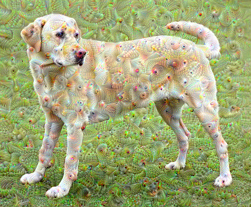
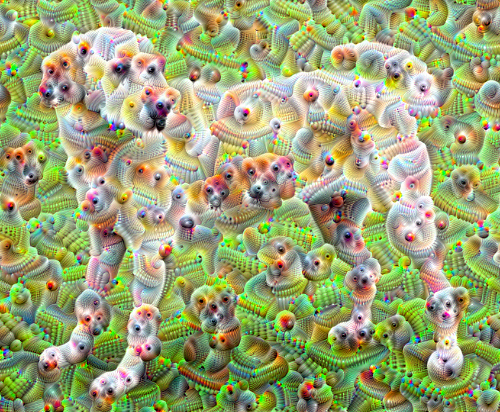
dream_img = run_deep_dream_simple(img=original_img,
                                  steps=100, step_size=0.01)
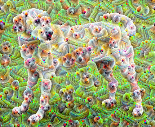
इसे एक सप्तक ऊपर लेना
बहुत अच्छा है, लेकिन इस पहले प्रयास में कुछ समस्याएं हैं:
- आउटपुट शोर है (इसे
tf.image.total_variationनुकसान के साथ संबोधित किया जा सकता है)। - छवि कम संकल्प है।
- पैटर्न ऐसे दिखाई देते हैं जैसे वे सभी एक ही ग्रैन्युलैरिटी पर हो रहे हों।
एक दृष्टिकोण जो इन सभी समस्याओं का समाधान करता है, वह है विभिन्न पैमानों पर क्रमिक आरोहण लागू करना। यह छोटे पैमाने पर उत्पन्न पैटर्न को उच्च पैमाने पर पैटर्न में शामिल करने और अतिरिक्त विवरण के साथ भरने की अनुमति देगा।
ऐसा करने के लिए आप पिछले ग्रेडिएंट चढ़ाई दृष्टिकोण का प्रदर्शन कर सकते हैं, फिर छवि के आकार को बढ़ा सकते हैं (जिसे एक सप्तक कहा जाता है), और इस प्रक्रिया को कई सप्तक के लिए दोहराएं।
import time
start = time.time()

OCTAVE_SCALE = 1.30

img = tf.constant(np.array(original_img))
base_shape = tf.shape(img)[:-1]
float_base_shape = tf.cast(base_shape, tf.float32)

for n in range(-2, 3):
  new_shape = tf.cast(float_base_shape*(OCTAVE_SCALE**n), tf.int32)

  img = tf.image.resize(img, new_shape).numpy()

  img = run_deep_dream_simple(img=img, steps=50, step_size=0.01)

display.clear_output(wait=True)
img = tf.image.resize(img, base_shape)
img = tf.image.convert_image_dtype(img/255.0, dtype=tf.uint8)
show(img)

end = time.time()
end-start
6.38355278968811
वैकल्पिक: टाइल्स के साथ स्केलिंग
विचार करने वाली एक बात यह है कि जैसे-जैसे छवि आकार में बढ़ती है, वैसे-वैसे समय और स्मृति को ढाल गणना करने के लिए आवश्यक होगा। उपरोक्त सप्तक कार्यान्वयन बहुत बड़ी छवियों, या कई सप्तक पर काम नहीं करेगा।
इस समस्या से बचने के लिए आप छवि को टाइलों में विभाजित कर सकते हैं और प्रत्येक टाइल के लिए ग्रेडिएंट की गणना कर सकते हैं।
प्रत्येक टाइल की गणना से पहले छवि में यादृच्छिक बदलाव लागू करना टाइल सीम को प्रदर्शित होने से रोकता है।
यादृच्छिक बदलाव को लागू करके प्रारंभ करें:
def random_roll(img, maxroll):
  # Randomly shift the image to avoid tiled boundaries.
  shift = tf.random.uniform(shape=[2], minval=-maxroll, maxval=maxroll, dtype=tf.int32)
  img_rolled = tf.roll(img, shift=shift, axis=[0,1])
  return shift, img_rolled
shift, img_rolled = random_roll(np.array(original_img), 512)
show(img_rolled)
यहां पहले से परिभाषित deepdream फ़ंक्शन का टाइल वाला समतुल्य है:
class TiledGradients(tf.Module):
  def __init__(self, model):
    self.model = model

  @tf.function(
      input_signature=(
        tf.TensorSpec(shape=[None,None,3], dtype=tf.float32),
        tf.TensorSpec(shape=[2], dtype=tf.int32),
        tf.TensorSpec(shape=[], dtype=tf.int32),)
  )
  def __call__(self, img, img_size, tile_size=512):
    shift, img_rolled = random_roll(img, tile_size)

    # Initialize the image gradients to zero.
    gradients = tf.zeros_like(img_rolled)

    # Skip the last tile, unless there's only one tile.
    xs = tf.range(0, img_size[1], tile_size)[:-1]
    if not tf.cast(len(xs), bool):
      xs = tf.constant([0])
    ys = tf.range(0, img_size[0], tile_size)[:-1]
    if not tf.cast(len(ys), bool):
      ys = tf.constant([0])

    for x in xs:
      for y in ys:
        # Calculate the gradients for this tile.
        with tf.GradientTape() as tape:
          # This needs gradients relative to `img_rolled`.
          # `GradientTape` only watches `tf.Variable`s by default.
          tape.watch(img_rolled)

          # Extract a tile out of the image.
          img_tile = img_rolled[y:y+tile_size, x:x+tile_size]
          loss = calc_loss(img_tile, self.model)

        # Update the image gradients for this tile.
        gradients = gradients + tape.gradient(loss, img_rolled)

    # Undo the random shift applied to the image and its gradients.
    gradients = tf.roll(gradients, shift=-shift, axis=[0,1])

    # Normalize the gradients.
    gradients /= tf.math.reduce_std(gradients) + 1e-8

    return gradients
get_tiled_gradients = TiledGradients(dream_model)
इसे एक साथ रखने से एक स्केलेबल, सप्तक-जागरूक डीपड्रीम कार्यान्वयन मिलता है:
def run_deep_dream_with_octaves(img, steps_per_octave=100, step_size=0.01,
                                octaves=range(-2,3), octave_scale=1.3):
  base_shape = tf.shape(img)
  img = tf.keras.utils.img_to_array(img)
  img = tf.keras.applications.inception_v3.preprocess_input(img)

  initial_shape = img.shape[:-1]
  img = tf.image.resize(img, initial_shape)
  for octave in octaves:
    # Scale the image based on the octave
    new_size = tf.cast(tf.convert_to_tensor(base_shape[:-1]), tf.float32)*(octave_scale**octave)
    new_size = tf.cast(new_size, tf.int32)
    img = tf.image.resize(img, new_size)

    for step in range(steps_per_octave):
      gradients = get_tiled_gradients(img, new_size)
      img = img + gradients*step_size
      img = tf.clip_by_value(img, -1, 1)

      if step % 10 == 0:
        display.clear_output(wait=True)
        show(deprocess(img))
        print ("Octave {}, Step {}".format(octave, step))

  result = deprocess(img)
  return result
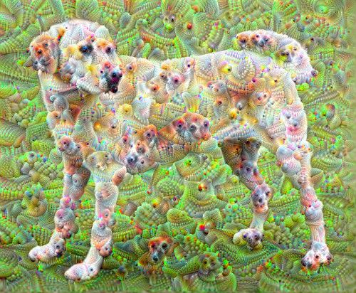
img = run_deep_dream_with_octaves(img=original_img, step_size=0.01)

display.clear_output(wait=True)
img = tf.image.resize(img, base_shape)
img = tf.image.convert_image_dtype(img/255.0, dtype=tf.uint8)
show(img)
काफी बेहतर! अपनी डीपड्रीम-एड छवि कैसे दिखती है, इसे बदलने के लिए ऑक्टेव्स, ऑक्टेव स्केल और सक्रिय परतों की संख्या के साथ खेलें।
पाठकों को TensorFlow Lucid में भी रुचि हो सकती है जो तंत्रिका नेटवर्क की कल्पना और व्याख्या करने के लिए इस ट्यूटोरियल में पेश किए गए विचारों पर विस्तार करता है।