
|
|
|
 View source on GitHub View source on GitHub
|
|
This tutorial demonstrates text classification starting from plain text files stored on disk. You'll train a binary classifier to perform sentiment analysis on an IMDB dataset. At the end of the notebook, there is an exercise for you to try, in which you'll train a multi-class classifier to predict the tag for a programming question on Stack Overflow.
import matplotlib.pyplot as plt
import os
import re
import shutil
import string
import tensorflow as tf

from tensorflow.keras import layers
from tensorflow.keras import losses
2024-08-31 01:24:31.567437: E external/local_xla/xla/stream_executor/cuda/cuda_fft.cc:485] Unable to register cuFFT factory: Attempting to register factory for plugin cuFFT when one has already been registered
2024-08-31 01:24:31.588777: E external/local_xla/xla/stream_executor/cuda/cuda_dnn.cc:8454] Unable to register cuDNN factory: Attempting to register factory for plugin cuDNN when one has already been registered
2024-08-31 01:24:31.595223: E external/local_xla/xla/stream_executor/cuda/cuda_blas.cc:1452] Unable to register cuBLAS factory: Attempting to register factory for plugin cuBLAS when one has already been registered
print(tf.__version__)
2.17.0
Sentiment analysis
This notebook trains a sentiment analysis model to classify movie reviews as positive or negative, based on the text of the review. This is an example of binary—or two-class—classification, an important and widely applicable kind of machine learning problem.
You'll use the Large Movie Review Dataset that contains the text of 50,000 movie reviews from the Internet Movie Database. These are split into 25,000 reviews for training and 25,000 reviews for testing. The training and testing sets are balanced, meaning they contain an equal number of positive and negative reviews.
Download and explore the IMDB dataset
Let's download and extract the dataset, then explore the directory structure.
url = "https://ai.stanford.edu/~amaas/data/sentiment/aclImdb_v1.tar.gz"

dataset = tf.keras.utils.get_file("aclImdb_v1", url,
                                    untar=True, cache_dir='.',
                                    cache_subdir='')

dataset_dir = os.path.join(os.path.dirname(dataset), 'aclImdb')
Downloading data from https://ai.stanford.edu/~amaas/data/sentiment/aclImdb_v1.tar.gz
84125825/84125825 ━━━━━━━━━━━━━━━━━━━━ 5s 0us/step
os.listdir(dataset_dir)
['train', 'README', 'imdbEr.txt', 'test', 'imdb.vocab']
train_dir = os.path.join(dataset_dir, 'train')
os.listdir(train_dir)
['unsupBow.feat',
 'urls_unsup.txt',
 'pos',
 'neg',
 'urls_neg.txt',
 'labeledBow.feat',
 'unsup',
 'urls_pos.txt']
The aclImdb/train/pos and aclImdb/train/neg directories contain many text files, each of which is a single movie review. Let's take a look at one of them.
sample_file = os.path.join(train_dir, 'pos/1181_9.txt')
with open(sample_file) as f:
  print(f.read())
Rachel Griffiths writes and directs this award winning short film. A heartwarming story about coping with grief and cherishing the memory of those we've loved and lost. Although, only 15 minutes long, Griffiths manages to capture so much emotion and truth onto film in the short space of time. Bud Tingwell gives a touching performance as Will, a widower struggling to cope with his wife's death. Will is confronted by the harsh reality of loneliness and helplessness as he proceeds to take care of Ruth's pet cow, Tulip. The film displays the grief and responsibility one feels for those they have loved and lost. Good cinematography, great direction, and superbly acted. It will bring tears to all those who have lost a loved one, and survived.
Load the dataset
Next, you will load the data off disk and prepare it into a format suitable for training. To do so, you will use the helpful text_dataset_from_directory utility, which expects a directory structure as follows.
main_directory/
...class_a/
......a_text_1.txt
......a_text_2.txt
...class_b/
......b_text_1.txt
......b_text_2.txt
To prepare a dataset for binary classification, you will need two folders on disk, corresponding to class_a and class_b. These will be the positive and negative movie reviews, which can be found in aclImdb/train/pos and aclImdb/train/neg. As the IMDB dataset contains additional folders, you will remove them before using this utility.
remove_dir = os.path.join(train_dir, 'unsup')
shutil.rmtree(remove_dir)
Next, you will use the text_dataset_from_directory utility to create a labeled tf.data.Dataset. tf.data is a powerful collection of tools for working with data.
When running a machine learning experiment, it is a best practice to divide your dataset into three splits: train, validation, and test.
The IMDB dataset has already been divided into train and test, but it lacks a validation set. Let's create a validation set using an 80:20 split of the training data by using the validation_split argument below.
batch_size = 32
seed = 42

raw_train_ds = tf.keras.utils.text_dataset_from_directory(
    'aclImdb/train',
    batch_size=batch_size,
    validation_split=0.2,
    subset='training',
    seed=seed)
Found 25000 files belonging to 2 classes.
Using 20000 files for training.
WARNING: All log messages before absl::InitializeLog() is called are written to STDERR
I0000 00:00:1725067500.786030   10188 cuda_executor.cc:1015] successful NUMA node read from SysFS had negative value (-1), but there must be at least one NUMA node, so returning NUMA node zero. See more at https://github.com/torvalds/linux/blob/v6.0/Documentation/ABI/testing/sysfs-bus-pci#L344-L355
I0000 00:00:1725067500.789584   10188 cuda_executor.cc:1015] successful NUMA node read from SysFS had negative value (-1), but there must be at least one NUMA node, so returning NUMA node zero. See more at https://github.com/torvalds/linux/blob/v6.0/Documentation/ABI/testing/sysfs-bus-pci#L344-L355
I0000 00:00:1725067500.793317   10188 cuda_executor.cc:1015] successful NUMA node read from SysFS had negative value (-1), but there must be at least one NUMA node, so returning NUMA node zero. See more at https://github.com/torvalds/linux/blob/v6.0/Documentation/ABI/testing/sysfs-bus-pci#L344-L355
I0000 00:00:1725067500.796882   10188 cuda_executor.cc:1015] successful NUMA node read from SysFS had negative value (-1), but there must be at least one NUMA node, so returning NUMA node zero. See more at https://github.com/torvalds/linux/blob/v6.0/Documentation/ABI/testing/sysfs-bus-pci#L344-L355
I0000 00:00:1725067500.808405   10188 cuda_executor.cc:1015] successful NUMA node read from SysFS had negative value (-1), but there must be at least one NUMA node, so returning NUMA node zero. See more at https://github.com/torvalds/linux/blob/v6.0/Documentation/ABI/testing/sysfs-bus-pci#L344-L355
I0000 00:00:1725067500.811533   10188 cuda_executor.cc:1015] successful NUMA node read from SysFS had negative value (-1), but there must be at least one NUMA node, so returning NUMA node zero. See more at https://github.com/torvalds/linux/blob/v6.0/Documentation/ABI/testing/sysfs-bus-pci#L344-L355
I0000 00:00:1725067500.815065   10188 cuda_executor.cc:1015] successful NUMA node read from SysFS had negative value (-1), but there must be at least one NUMA node, so returning NUMA node zero. See more at https://github.com/torvalds/linux/blob/v6.0/Documentation/ABI/testing/sysfs-bus-pci#L344-L355
I0000 00:00:1725067500.818427   10188 cuda_executor.cc:1015] successful NUMA node read from SysFS had negative value (-1), but there must be at least one NUMA node, so returning NUMA node zero. See more at https://github.com/torvalds/linux/blob/v6.0/Documentation/ABI/testing/sysfs-bus-pci#L344-L355
I0000 00:00:1725067500.821917   10188 cuda_executor.cc:1015] successful NUMA node read from SysFS had negative value (-1), but there must be at least one NUMA node, so returning NUMA node zero. See more at https://github.com/torvalds/linux/blob/v6.0/Documentation/ABI/testing/sysfs-bus-pci#L344-L355
I0000 00:00:1725067500.825170   10188 cuda_executor.cc:1015] successful NUMA node read from SysFS had negative value (-1), but there must be at least one NUMA node, so returning NUMA node zero. See more at https://github.com/torvalds/linux/blob/v6.0/Documentation/ABI/testing/sysfs-bus-pci#L344-L355
I0000 00:00:1725067500.828605   10188 cuda_executor.cc:1015] successful NUMA node read from SysFS had negative value (-1), but there must be at least one NUMA node, so returning NUMA node zero. See more at https://github.com/torvalds/linux/blob/v6.0/Documentation/ABI/testing/sysfs-bus-pci#L344-L355
I0000 00:00:1725067500.832057   10188 cuda_executor.cc:1015] successful NUMA node read from SysFS had negative value (-1), but there must be at least one NUMA node, so returning NUMA node zero. See more at https://github.com/torvalds/linux/blob/v6.0/Documentation/ABI/testing/sysfs-bus-pci#L344-L355
I0000 00:00:1725067502.069943   10188 cuda_executor.cc:1015] successful NUMA node read from SysFS had negative value (-1), but there must be at least one NUMA node, so returning NUMA node zero. See more at https://github.com/torvalds/linux/blob/v6.0/Documentation/ABI/testing/sysfs-bus-pci#L344-L355
I0000 00:00:1725067502.072028   10188 cuda_executor.cc:1015] successful NUMA node read from SysFS had negative value (-1), but there must be at least one NUMA node, so returning NUMA node zero. See more at https://github.com/torvalds/linux/blob/v6.0/Documentation/ABI/testing/sysfs-bus-pci#L344-L355
I0000 00:00:1725067502.074019   10188 cuda_executor.cc:1015] successful NUMA node read from SysFS had negative value (-1), but there must be at least one NUMA node, so returning NUMA node zero. See more at https://github.com/torvalds/linux/blob/v6.0/Documentation/ABI/testing/sysfs-bus-pci#L344-L355
I0000 00:00:1725067502.076000   10188 cuda_executor.cc:1015] successful NUMA node read from SysFS had negative value (-1), but there must be at least one NUMA node, so returning NUMA node zero. See more at https://github.com/torvalds/linux/blob/v6.0/Documentation/ABI/testing/sysfs-bus-pci#L344-L355
I0000 00:00:1725067502.078012   10188 cuda_executor.cc:1015] successful NUMA node read from SysFS had negative value (-1), but there must be at least one NUMA node, so returning NUMA node zero. See more at https://github.com/torvalds/linux/blob/v6.0/Documentation/ABI/testing/sysfs-bus-pci#L344-L355
I0000 00:00:1725067502.079954   10188 cuda_executor.cc:1015] successful NUMA node read from SysFS had negative value (-1), but there must be at least one NUMA node, so returning NUMA node zero. See more at https://github.com/torvalds/linux/blob/v6.0/Documentation/ABI/testing/sysfs-bus-pci#L344-L355
I0000 00:00:1725067502.081839   10188 cuda_executor.cc:1015] successful NUMA node read from SysFS had negative value (-1), but there must be at least one NUMA node, so returning NUMA node zero. See more at https://github.com/torvalds/linux/blob/v6.0/Documentation/ABI/testing/sysfs-bus-pci#L344-L355
I0000 00:00:1725067502.083730   10188 cuda_executor.cc:1015] successful NUMA node read from SysFS had negative value (-1), but there must be at least one NUMA node, so returning NUMA node zero. See more at https://github.com/torvalds/linux/blob/v6.0/Documentation/ABI/testing/sysfs-bus-pci#L344-L355
I0000 00:00:1725067502.085640   10188 cuda_executor.cc:1015] successful NUMA node read from SysFS had negative value (-1), but there must be at least one NUMA node, so returning NUMA node zero. See more at https://github.com/torvalds/linux/blob/v6.0/Documentation/ABI/testing/sysfs-bus-pci#L344-L355
I0000 00:00:1725067502.087598   10188 cuda_executor.cc:1015] successful NUMA node read from SysFS had negative value (-1), but there must be at least one NUMA node, so returning NUMA node zero. See more at https://github.com/torvalds/linux/blob/v6.0/Documentation/ABI/testing/sysfs-bus-pci#L344-L355
I0000 00:00:1725067502.089508   10188 cuda_executor.cc:1015] successful NUMA node read from SysFS had negative value (-1), but there must be at least one NUMA node, so returning NUMA node zero. See more at https://github.com/torvalds/linux/blob/v6.0/Documentation/ABI/testing/sysfs-bus-pci#L344-L355
I0000 00:00:1725067502.091411   10188 cuda_executor.cc:1015] successful NUMA node read from SysFS had negative value (-1), but there must be at least one NUMA node, so returning NUMA node zero. See more at https://github.com/torvalds/linux/blob/v6.0/Documentation/ABI/testing/sysfs-bus-pci#L344-L355
I0000 00:00:1725067502.130441   10188 cuda_executor.cc:1015] successful NUMA node read from SysFS had negative value (-1), but there must be at least one NUMA node, so returning NUMA node zero. See more at https://github.com/torvalds/linux/blob/v6.0/Documentation/ABI/testing/sysfs-bus-pci#L344-L355
I0000 00:00:1725067502.132468   10188 cuda_executor.cc:1015] successful NUMA node read from SysFS had negative value (-1), but there must be at least one NUMA node, so returning NUMA node zero. See more at https://github.com/torvalds/linux/blob/v6.0/Documentation/ABI/testing/sysfs-bus-pci#L344-L355
I0000 00:00:1725067502.134399   10188 cuda_executor.cc:1015] successful NUMA node read from SysFS had negative value (-1), but there must be at least one NUMA node, so returning NUMA node zero. See more at https://github.com/torvalds/linux/blob/v6.0/Documentation/ABI/testing/sysfs-bus-pci#L344-L355
I0000 00:00:1725067502.136340   10188 cuda_executor.cc:1015] successful NUMA node read from SysFS had negative value (-1), but there must be at least one NUMA node, so returning NUMA node zero. See more at https://github.com/torvalds/linux/blob/v6.0/Documentation/ABI/testing/sysfs-bus-pci#L344-L355
I0000 00:00:1725067502.138734   10188 cuda_executor.cc:1015] successful NUMA node read from SysFS had negative value (-1), but there must be at least one NUMA node, so returning NUMA node zero. See more at https://github.com/torvalds/linux/blob/v6.0/Documentation/ABI/testing/sysfs-bus-pci#L344-L355
I0000 00:00:1725067502.140671   10188 cuda_executor.cc:1015] successful NUMA node read from SysFS had negative value (-1), but there must be at least one NUMA node, so returning NUMA node zero. See more at https://github.com/torvalds/linux/blob/v6.0/Documentation/ABI/testing/sysfs-bus-pci#L344-L355
I0000 00:00:1725067502.142572   10188 cuda_executor.cc:1015] successful NUMA node read from SysFS had negative value (-1), but there must be at least one NUMA node, so returning NUMA node zero. See more at https://github.com/torvalds/linux/blob/v6.0/Documentation/ABI/testing/sysfs-bus-pci#L344-L355
I0000 00:00:1725067502.144502   10188 cuda_executor.cc:1015] successful NUMA node read from SysFS had negative value (-1), but there must be at least one NUMA node, so returning NUMA node zero. See more at https://github.com/torvalds/linux/blob/v6.0/Documentation/ABI/testing/sysfs-bus-pci#L344-L355
I0000 00:00:1725067502.146416   10188 cuda_executor.cc:1015] successful NUMA node read from SysFS had negative value (-1), but there must be at least one NUMA node, so returning NUMA node zero. See more at https://github.com/torvalds/linux/blob/v6.0/Documentation/ABI/testing/sysfs-bus-pci#L344-L355
I0000 00:00:1725067502.150429   10188 cuda_executor.cc:1015] successful NUMA node read from SysFS had negative value (-1), but there must be at least one NUMA node, so returning NUMA node zero. See more at https://github.com/torvalds/linux/blob/v6.0/Documentation/ABI/testing/sysfs-bus-pci#L344-L355
I0000 00:00:1725067502.152777   10188 cuda_executor.cc:1015] successful NUMA node read from SysFS had negative value (-1), but there must be at least one NUMA node, so returning NUMA node zero. See more at https://github.com/torvalds/linux/blob/v6.0/Documentation/ABI/testing/sysfs-bus-pci#L344-L355
I0000 00:00:1725067502.155044   10188 cuda_executor.cc:1015] successful NUMA node read from SysFS had negative value (-1), but there must be at least one NUMA node, so returning NUMA node zero. See more at https://github.com/torvalds/linux/blob/v6.0/Documentation/ABI/testing/sysfs-bus-pci#L344-L355
As you can see above, there are 25,000 examples in the training folder, of which you will use 80% (or 20,000) for training. As you will see in a moment, you can train a model by passing a dataset directly to model.fit. If you're new to tf.data, you can also iterate over the dataset and print out a few examples as follows.
for text_batch, label_batch in raw_train_ds.take(1):
  for i in range(3):
    print("Review", text_batch.numpy()[i])
    print("Label", label_batch.numpy()[i])
Review b'"Pandemonium" is a horror movie spoof that comes off more stupid than funny. Believe me when I tell you, I love comedies. Especially comedy spoofs. "Airplane", "The Naked Gun" trilogy, "Blazing Saddles", "High Anxiety", and "Spaceballs" are some of my favorite comedies that spoof a particular genre. "Pandemonium" is not up there with those films. Most of the scenes in this movie had me sitting there in stunned silence because the movie wasn\'t all that funny. There are a few laughs in the film, but when you watch a comedy, you expect to laugh a lot more than a few times and that\'s all this film has going for it. Geez, "Scream" had more laughs than this film and that was more of a horror film. How bizarre is that?<br /><br />*1/2 (out of four)'
Label 0
Review b"David Mamet is a very interesting and a very un-equal director. His first movie 'House of Games' was the one I liked best, and it set a series of films with characters whose perspective of life changes as they get into complicated situations, and so does the perspective of the viewer.<br /><br />So is 'Homicide' which from the title tries to set the mind of the viewer to the usual crime drama. The principal characters are two cops, one Jewish and one Irish who deal with a racially charged area. The murder of an old Jewish shop owner who proves to be an ancient veteran of the Israeli Independence war triggers the Jewish identity in the mind and heart of the Jewish detective.<br /><br />This is were the flaws of the film are the more obvious. The process of awakening is theatrical and hard to believe, the group of Jewish militants is operatic, and the way the detective eventually walks to the final violent confrontation is pathetic. The end of the film itself is Mamet-like smart, but disappoints from a human emotional perspective.<br /><br />Joe Mantegna and William Macy give strong performances, but the flaws of the story are too evident to be easily compensated."
Label 0
Review b'Great documentary about the lives of NY firefighters during the worst terrorist attack of all time.. That reason alone is why this should be a must see collectors item.. What shocked me was not only the attacks, but the"High Fat Diet" and physical appearance of some of these firefighters. I think a lot of Doctors would agree with me that,in the physical shape they were in, some of these firefighters would NOT of made it to the 79th floor carrying over 60 lbs of gear. Having said that i now have a greater respect for firefighters and i realize becoming a firefighter is a life altering job. The French have a history of making great documentary\'s and that is what this is, a Great Documentary.....'
Label 1
Notice the reviews contain raw text (with punctuation and occasional HTML tags like <br/>). You will show how to handle these in the following section.
The labels are 0 or 1. To see which of these correspond to positive and negative movie reviews, you can check the class_names property on the dataset.
print("Label 0 corresponds to", raw_train_ds.class_names[0])
print("Label 1 corresponds to", raw_train_ds.class_names[1])
Label 0 corresponds to neg
Label 1 corresponds to pos
Next, you will create a validation and test dataset. You will use the remaining 5,000 reviews from the training set for validation.
raw_val_ds = tf.keras.utils.text_dataset_from_directory(
    'aclImdb/train',
    batch_size=batch_size,
    validation_split=0.2,
    subset='validation',
    seed=seed)
Found 25000 files belonging to 2 classes.
Using 5000 files for validation.
raw_test_ds = tf.keras.utils.text_dataset_from_directory(
    'aclImdb/test',
    batch_size=batch_size)
Found 25000 files belonging to 2 classes.
Prepare the dataset for training
Next, you will standardize, tokenize, and vectorize the data using the helpful tf.keras.layers.TextVectorization layer.
Standardization refers to preprocessing the text, typically to remove punctuation or HTML elements to simplify the dataset. Tokenization refers to splitting strings into tokens (for example, splitting a sentence into individual words, by splitting on whitespace). Vectorization refers to converting tokens into numbers so they can be fed into a neural network. All of these tasks can be accomplished with this layer.
As you saw above, the reviews contain various HTML tags like <br />. These tags will not be removed by the default standardizer in the TextVectorization layer (which converts text to lowercase and strips punctuation by default, but doesn't strip HTML). You will write a custom standardization function to remove the HTML.
def custom_standardization(input_data):
  lowercase = tf.strings.lower(input_data)
  stripped_html = tf.strings.regex_replace(lowercase, '<br />', ' ')
  return tf.strings.regex_replace(stripped_html,
                                  '[%s]' % re.escape(string.punctuation),
                                  '')
Next, you will create a TextVectorization layer. You will use this layer to standardize, tokenize, and vectorize our data. You set the output_mode to int to create unique integer indices for each token.
Note that you're using the default split function, and the custom standardization function you defined above. You'll also define some constants for the model, like an explicit maximum sequence_length, which will cause the layer to pad or truncate sequences to exactly sequence_length values.
max_features = 10000
sequence_length = 250

vectorize_layer = layers.TextVectorization(
    standardize=custom_standardization,
    max_tokens=max_features,
    output_mode='int',
    output_sequence_length=sequence_length)
Next, you will call adapt to fit the state of the preprocessing layer to the dataset. This will cause the model to build an index of strings to integers.
# Make a text-only dataset (without labels), then call adapt
train_text = raw_train_ds.map(lambda x, y: x)
vectorize_layer.adapt(train_text)
Let's create a function to see the result of using this layer to preprocess some data.
def vectorize_text(text, label):
  text = tf.expand_dims(text, -1)
  return vectorize_layer(text), label
# retrieve a batch (of 32 reviews and labels) from the dataset
text_batch, label_batch = next(iter(raw_train_ds))
first_review, first_label = text_batch[0], label_batch[0]
print("Review", first_review)
print("Label", raw_train_ds.class_names[first_label])
print("Vectorized review", vectorize_text(first_review, first_label))
Review tf.Tensor(b'Silent Night, Deadly Night 5 is the very last of the series, and like part 4, it\'s unrelated to the first three except by title and the fact that it\'s a Christmas-themed horror flick.<br /><br />Except to the oblivious, there\'s some obvious things going on here...Mickey Rooney plays a toymaker named Joe Petto and his creepy son\'s name is Pino. Ring a bell, anyone? Now, a little boy named Derek heard a knock at the door one evening, and opened it to find a present on the doorstep for him. Even though it said "don\'t open till Christmas", he begins to open it anyway but is stopped by his dad, who scolds him and sends him to bed, and opens the gift himself. Inside is a little red ball that sprouts Santa arms and a head, and proceeds to kill dad. Oops, maybe he should have left well-enough alone. Of course Derek is then traumatized by the incident since he watched it from the stairs, but he doesn\'t grow up to be some killer Santa, he just stops talking.<br /><br />There\'s a mysterious stranger lurking around, who seems very interested in the toys that Joe Petto makes. We even see him buying a bunch when Derek\'s mom takes him to the store to find a gift for him to bring him out of his trauma. And what exactly is this guy doing? Well, we\'re not sure but he does seem to be taking these toys apart to see what makes them tick. He does keep his landlord from evicting him by promising him to pay him in cash the next day and presents him with a "Larry the Larvae" toy for his kid, but of course "Larry" is not a good toy and gets out of the box in the car and of course, well, things aren\'t pretty.<br /><br />Anyway, eventually what\'s going on with Joe Petto and Pino is of course revealed, and as with the old story, Pino is not a "real boy". Pino is probably even more agitated and naughty because he suffers from "Kenitalia" (a smooth plastic crotch) so that could account for his evil ways. And the identity of the lurking stranger is revealed too, and there\'s even kind of a happy ending of sorts. Whee.<br /><br />A step up from part 4, but not much of one. Again, Brian Yuzna is involved, and Screaming Mad George, so some decent special effects, but not enough to make this great. A few leftovers from part 4 are hanging around too, like Clint Howard and Neith Hunter, but that doesn\'t really make any difference. Anyway, I now have seeing the whole series out of my system. Now if I could get some of it out of my brain. 4 out of 5.', shape=(), dtype=string)
Label neg
Vectorized review (<tf.Tensor: shape=(1, 250), dtype=int64, numpy=
array([[1287,  313, 2380,  313,  661,    7,    2,   52,  229,    5,    2,
         200,    3,   38,  170,  669,   29, 5492,    6,    2,   83,  297,
         549,   32,  410,    3,    2,  186,   12,   29,    4,    1,  191,
         510,  549,    6,    2, 8229,  212,   46,  576,  175,  168,   20,
           1, 5361,  290,    4,    1,  761,  969,    1,    3,   24,  935,
        2271,  393,    7,    1, 1675,    4, 3747,  250,  148,    4,  112,
         436,  761, 3529,  548,    4, 3633,   31,    2, 1331,   28, 2096,
           3, 2912,    9,    6,  163,    4, 1006,   20,    2,    1,   15,
          85,   53,  147,    9,  292,   89,  959, 2314,  984,   27,  762,
           6,  959,    9,  564,   18,    7, 2140,   32,   24, 1254,   36,
           1,   85,    3, 3298,   85,    6, 1410,    3, 1936,    2, 3408,
         301,  965,    7,    4,  112,  740, 1977,   12,    1, 2014, 2772,
           3,    4,  428,    3, 5177,    6,  512, 1254,    1,  278,   27,
         139,   25,  308,    1,  579,    5,  259, 3529,    7,   92, 8981,
          32,    2, 3842,  230,   27,  289,    9,   35,    2, 5712,   18,
          27,  144, 2166,   56,    6,   26,   46,  466, 2014,   27,   40,
        2745,  657,  212,    4, 1376, 3002, 7080,  183,   36,  180,   52,
         920,    8,    2, 4028,   12,  969,    1,  158,   71,   53,   67,
          85, 2754,    4,  734,   51,    1, 1611,  294,   85,    6,    2,
        1164,    6,  163,    4, 3408,   15,   85,    6,  717,   85,   44,
           5,   24, 7158,    3,   48,  604,    7,   11,  225,  384,   73,
          65,   21,  242,   18,   27,  120,  295,    6,   26,  667,  129,
        4028,  948,    6,   67,   48,  158,   93,    1]])>, <tf.Tensor: shape=(), dtype=int32, numpy=0>)
As you can see above, each token has been replaced by an integer. You can lookup the token (string) that each integer corresponds to by calling .get_vocabulary() on the layer.
print("1287 ---> ",vectorize_layer.get_vocabulary()[1287])
print(" 313 ---> ",vectorize_layer.get_vocabulary()[313])
print('Vocabulary size: {}'.format(len(vectorize_layer.get_vocabulary())))
1287 --->  silent
 313 --->  night
Vocabulary size: 10000
You are nearly ready to train your model. As a final preprocessing step, you will apply the TextVectorization layer you created earlier to the train, validation, and test dataset.
train_ds = raw_train_ds.map(vectorize_text)
val_ds = raw_val_ds.map(vectorize_text)
test_ds = raw_test_ds.map(vectorize_text)
Configure the dataset for performance
These are two important methods you should use when loading data to make sure that I/O does not become blocking.
.cache() keeps data in memory after it's loaded off disk. This will ensure the dataset does not become a bottleneck while training your model. If your dataset is too large to fit into memory, you can also use this method to create a performant on-disk cache, which is more efficient to read than many small files.
.prefetch() overlaps data preprocessing and model execution while training.
You can learn more about both methods, as well as how to cache data to disk in the data performance guide.
AUTOTUNE = tf.data.AUTOTUNE

train_ds = train_ds.cache().prefetch(buffer_size=AUTOTUNE)
val_ds = val_ds.cache().prefetch(buffer_size=AUTOTUNE)
test_ds = test_ds.cache().prefetch(buffer_size=AUTOTUNE)
Create the model
It's time to create your neural network:
embedding_dim = 16
model = tf.keras.Sequential([
  layers.Embedding(max_features, embedding_dim),
  layers.Dropout(0.2),
  layers.GlobalAveragePooling1D(),
  layers.Dropout(0.2),
  layers.Dense(1, activation='sigmoid')])

model.summary()
The layers are stacked sequentially to build the classifier:
- The first layer is an
Embeddinglayer. This layer takes the integer-encoded reviews and looks up an embedding vector for each word-index. These vectors are learned as the model trains. The vectors add a dimension to the output array. The resulting dimensions are:(batch, sequence, embedding). To learn more about embeddings, check out the Word embeddings tutorial. - Next, a
GlobalAveragePooling1Dlayer returns a fixed-length output vector for each example by averaging over the sequence dimension. This allows the model to handle input of variable length, in the simplest way possible. - The last layer is densely connected with a single output node.
Loss function and optimizer
A model needs a loss function and an optimizer for training. Since this is a binary classification problem and the model outputs a probability (a single-unit layer with a sigmoid activation), you'll use losses.BinaryCrossentropy loss function.
Now, configure the model to use an optimizer and a loss function:
model.compile(loss=losses.BinaryCrossentropy(),
              optimizer='adam',
              metrics=[tf.metrics.BinaryAccuracy(threshold=0.5)])
Train the model
You will train the model by passing the dataset object to the fit method.
epochs = 10
history = model.fit(
    train_ds,
    validation_data=val_ds,
    epochs=epochs)
Epoch 1/10
WARNING: All log messages before absl::InitializeLog() is called are written to STDERR
I0000 00:00:1725067511.995924   10397 service.cc:146] XLA service 0x7faa280080c0 initialized for platform CUDA (this does not guarantee that XLA will be used). Devices:
I0000 00:00:1725067511.995953   10397 service.cc:154]   StreamExecutor device (0): Tesla T4, Compute Capability 7.5
I0000 00:00:1725067511.995957   10397 service.cc:154]   StreamExecutor device (1): Tesla T4, Compute Capability 7.5
I0000 00:00:1725067511.995960   10397 service.cc:154]   StreamExecutor device (2): Tesla T4, Compute Capability 7.5
I0000 00:00:1725067511.995963   10397 service.cc:154]   StreamExecutor device (3): Tesla T4, Compute Capability 7.5
89/625 ━━━━━━━━━━━━━━━━━━━━ 0s 2ms/step - binary_accuracy: 0.5286 - loss: 0.6921
I0000 00:00:1725067513.261163   10397 device_compiler.h:188] Compiled cluster using XLA!  This line is logged at most once for the lifetime of the process.
625/625 ━━━━━━━━━━━━━━━━━━━━ 4s 3ms/step - binary_accuracy: 0.5878 - loss: 0.6801 - val_binary_accuracy: 0.7314 - val_loss: 0.6106
Epoch 2/10
625/625 ━━━━━━━━━━━━━━━━━━━━ 1s 1ms/step - binary_accuracy: 0.7592 - loss: 0.5773 - val_binary_accuracy: 0.8110 - val_loss: 0.4969
Epoch 3/10
625/625 ━━━━━━━━━━━━━━━━━━━━ 1s 1ms/step - binary_accuracy: 0.8232 - loss: 0.4648 - val_binary_accuracy: 0.8266 - val_loss: 0.4301
Epoch 4/10
625/625 ━━━━━━━━━━━━━━━━━━━━ 1s 1ms/step - binary_accuracy: 0.8496 - loss: 0.3929 - val_binary_accuracy: 0.8392 - val_loss: 0.3867
Epoch 5/10
625/625 ━━━━━━━━━━━━━━━━━━━━ 1s 1ms/step - binary_accuracy: 0.8693 - loss: 0.3467 - val_binary_accuracy: 0.8446 - val_loss: 0.3628
Epoch 6/10
625/625 ━━━━━━━━━━━━━━━━━━━━ 1s 1ms/step - binary_accuracy: 0.8814 - loss: 0.3142 - val_binary_accuracy: 0.8536 - val_loss: 0.3428
Epoch 7/10
625/625 ━━━━━━━━━━━━━━━━━━━━ 1s 1ms/step - binary_accuracy: 0.8930 - loss: 0.2889 - val_binary_accuracy: 0.8546 - val_loss: 0.3319
Epoch 8/10
625/625 ━━━━━━━━━━━━━━━━━━━━ 1s 1ms/step - binary_accuracy: 0.8986 - loss: 0.2689 - val_binary_accuracy: 0.8568 - val_loss: 0.3250
Epoch 9/10
625/625 ━━━━━━━━━━━━━━━━━━━━ 1s 1ms/step - binary_accuracy: 0.9079 - loss: 0.2515 - val_binary_accuracy: 0.8570 - val_loss: 0.3201
Epoch 10/10
625/625 ━━━━━━━━━━━━━━━━━━━━ 1s 1ms/step - binary_accuracy: 0.9118 - loss: 0.2379 - val_binary_accuracy: 0.8592 - val_loss: 0.3156
Evaluate the model
Let's see how the model performs. Two values will be returned. Loss (a number which represents our error, lower values are better), and accuracy.
loss, accuracy = model.evaluate(test_ds)

print("Loss: ", loss)
print("Accuracy: ", accuracy)
782/782 ━━━━━━━━━━━━━━━━━━━━ 1s 2ms/step - binary_accuracy: 0.8534 - loss: 0.3383
Loss:  0.33511972427368164
Accuracy:  0.8527200222015381
This fairly naive approach achieves an accuracy of about 86%.
Create a plot of accuracy and loss over time
model.fit() returns a History object that contains a dictionary with everything that happened during training:
history_dict = history.history
history_dict.keys()
dict_keys(['binary_accuracy', 'loss', 'val_binary_accuracy', 'val_loss'])
There are four entries: one for each monitored metric during training and validation. You can use these to plot the training and validation loss for comparison, as well as the training and validation accuracy:
acc = history_dict['binary_accuracy']
val_acc = history_dict['val_binary_accuracy']
loss = history_dict['loss']
val_loss = history_dict['val_loss']

epochs = range(1, len(acc) + 1)

# "bo" is for "blue dot"
plt.plot(epochs, loss, 'bo', label='Training loss')
# b is for "solid blue line"
plt.plot(epochs, val_loss, 'b', label='Validation loss')
plt.title('Training and validation loss')
plt.xlabel('Epochs')
plt.ylabel('Loss')
plt.legend()

plt.show()
plt.plot(epochs, acc, 'bo', label='Training acc')
plt.plot(epochs, val_acc, 'b', label='Validation acc')
plt.title('Training and validation accuracy')
plt.xlabel('Epochs')
plt.ylabel('Accuracy')
plt.legend(loc='lower right')

plt.show()
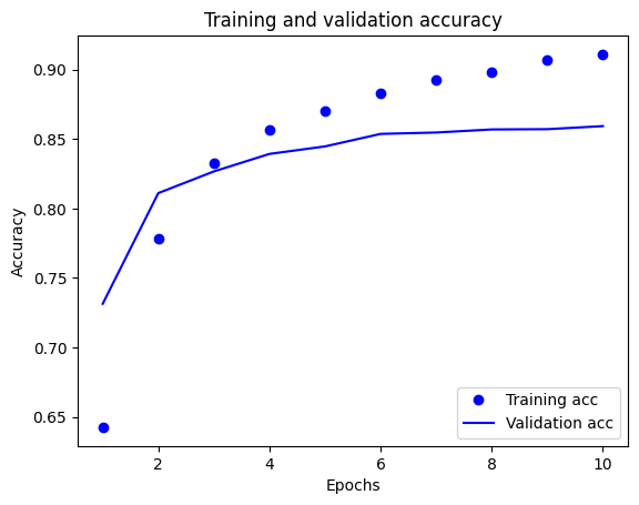
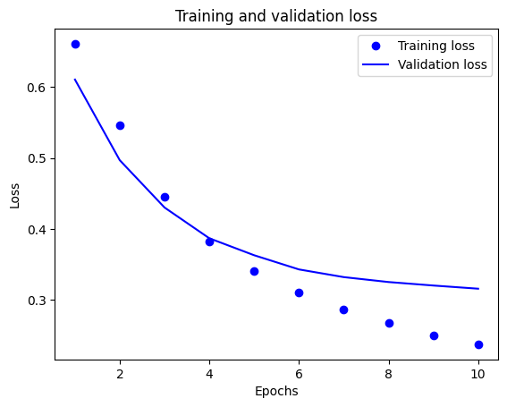
In this plot, the dots represent the training loss and accuracy, and the solid lines are the validation loss and accuracy.
Notice the training loss decreases with each epoch and the training accuracy increases with each epoch. This is expected when using a gradient descent optimization—it should minimize the desired quantity on every iteration.
This isn't the case for the validation loss and accuracy—they seem to peak before the training accuracy. This is an example of overfitting: the model performs better on the training data than it does on data it has never seen before. After this point, the model over-optimizes and learns representations specific to the training data that do not generalize to test data.
For this particular case, you could prevent overfitting by simply stopping the training when the validation accuracy is no longer increasing. One way to do so is to use the tf.keras.callbacks.EarlyStopping callback.
Export the model
In the code above, you applied the TextVectorization layer to the dataset before feeding text to the model. If you want to make your model capable of processing raw strings (for example, to simplify deploying it), you can include the TextVectorization layer inside your model. To do so, you can create a new model using the weights you just trained.
export_model = tf.keras.Sequential([
  vectorize_layer,
  model,
  layers.Activation('sigmoid')
])

export_model.compile(
    loss=losses.BinaryCrossentropy(from_logits=False), optimizer="adam", metrics=['accuracy']
)

# Test it with `raw_test_ds`, which yields raw strings
metrics = export_model.evaluate(raw_test_ds, return_dict=True)
print(metrics)
782/782 ━━━━━━━━━━━━━━━━━━━━ 4s 4ms/step - accuracy: 0.4997 - binary_accuracy: 0.0000e+00 - loss: 0.0000e+00
{'accuracy': 0.5000399947166443, 'binary_accuracy': 0.0, 'loss': 0.0}
Inference on new data
To get predictions for new examples, you can simply call model.predict().
examples = tf.constant([
  "The movie was great!",
  "The movie was okay.",
  "The movie was terrible..."
])

export_model.predict(examples)
1/1 ━━━━━━━━━━━━━━━━━━━━ 0s 148ms/step
array([[0.57763124],
       [0.5442707 ],
       [0.53183067]], dtype=float32)
Including the text preprocessing logic inside your model enables you to export a model for production that simplifies deployment, and reduces the potential for train/test skew.
There is a performance difference to keep in mind when choosing where to apply your TextVectorization layer. Using it outside of your model enables you to do asynchronous CPU processing and buffering of your data when training on GPU. So, if you're training your model on the GPU, you probably want to go with this option to get the best performance while developing your model, then switch to including the TextVectorization layer inside your model when you're ready to prepare for deployment.
Visit this tutorial to learn more about saving models.
Exercise: multi-class classification on Stack Overflow questions
This tutorial showed how to train a binary classifier from scratch on the IMDB dataset. As an exercise, you can modify this notebook to train a multi-class classifier to predict the tag of a programming question on Stack Overflow.
A dataset has been prepared for you to use containing the body of several thousand programming questions (for example, "How can I sort a dictionary by value in Python?") posted to Stack Overflow. Each of these is labeled with exactly one tag (either Python, CSharp, JavaScript, or Java). Your task is to take a question as input, and predict the appropriate tag, in this case, Python.
The dataset you will work with contains several thousand questions extracted from the much larger public Stack Overflow dataset on BigQuery, which contains more than 17 million posts.
After downloading the dataset, you will find it has a similar directory structure to the IMDB dataset you worked with previously:
train/
...python/
......0.txt
......1.txt
...javascript/
......0.txt
......1.txt
...csharp/
......0.txt
......1.txt
...java/
......0.txt
......1.txt
To complete this exercise, you should modify this notebook to work with the Stack Overflow dataset by making the following modifications:
At the top of your notebook, update the code that downloads the IMDB dataset with code to download the Stack Overflow dataset that has already been prepared. As the Stack Overflow dataset has a similar directory structure, you will not need to make many modifications.
Modify the last layer of your model to
Dense(4), as there are now four output classes.When compiling the model, change the loss to
tf.keras.losses.SparseCategoricalCrossentropy(from_logits=True). This is the correct loss function to use for a multi-class classification problem, when the labels for each class are integers (in this case, they can be 0, 1, 2, or 3). In addition, change the metrics tometrics=['accuracy'], since this is a multi-class classification problem (tf.metrics.BinaryAccuracyis only used for binary classifiers).When plotting accuracy over time, change
binary_accuracyandval_binary_accuracytoaccuracyandval_accuracy, respectively.Once these changes are complete, you will be able to train a multi-class classifier.
Learning more
This tutorial introduced text classification from scratch. To learn more about the text classification workflow in general, check out the Text classification guide from Google Developers.
# MIT License
#
# Copyright (c) 2017 François Chollet
#
# Permission is hereby granted, free of charge, to any person obtaining a
# copy of this software and associated documentation files (the "Software"),
# to deal in the Software without restriction, including without limitation
# the rights to use, copy, modify, merge, publish, distribute, sublicense,
# and/or sell copies of the Software, and to permit persons to whom the
# Software is furnished to do so, subject to the following conditions:
#
# The above copyright notice and this permission notice shall be included in
# all copies or substantial portions of the Software.
#
# THE SOFTWARE IS PROVIDED "AS IS", WITHOUT WARRANTY OF ANY KIND, EXPRESS OR
# IMPLIED, INCLUDING BUT NOT LIMITED TO THE WARRANTIES OF MERCHANTABILITY,
# FITNESS FOR A PARTICULAR PURPOSE AND NONINFRINGEMENT. IN NO EVENT SHALL
# THE AUTHORS OR COPYRIGHT HOLDERS BE LIABLE FOR ANY CLAIM, DAMAGES OR OTHER
# LIABILITY, WHETHER IN AN ACTION OF CONTRACT, TORT OR OTHERWISE, ARISING
# FROM, OUT OF OR IN CONNECTION WITH THE SOFTWARE OR THE USE OR OTHER
# DEALINGS IN THE SOFTWARE.