| | |  गिटहब पर देखें गिटहब पर देखें | | |
YAMNet एक गहरी शुद्ध कि 521 ऑडियो घटना की भविष्यवाणी है वर्गों से AudioSet-यूट्यूब कोष उस पर प्रशिक्षित किया गया था। यह रोजगार Mobilenet_v1 depthwise-वियोज्य घुमाव के वास्तुकला।
import tensorflow as tf
import tensorflow_hub as hub
import numpy as np
import csv

import matplotlib.pyplot as plt
from IPython.display import Audio
from scipy.io import wavfile
मॉडल को TensorFlow हब से लोड करें।
# Load the model.
model = hub.load('https://tfhub.dev/google/yamnet/1')
लेबल फ़ाइल मॉडल परिसंपत्तियों से लोड किया जाएगा और वर्तमान में है model.class_map_path() आप पर यह लोड होगा class_names चर।
# Find the name of the class with the top score when mean-aggregated across frames.
def class_names_from_csv(class_map_csv_text):
  """Returns list of class names corresponding to score vector."""
  class_names = []
  with tf.io.gfile.GFile(class_map_csv_text) as csvfile:
    reader = csv.DictReader(csvfile)
    for row in reader:
      class_names.append(row['display_name'])

  return class_names

class_map_path = model.class_map_path().numpy()
class_names = class_names_from_csv(class_map_path)
लोड किए गए ऑडियो को सत्यापित करने और परिवर्तित करने के लिए एक विधि जोड़ें उचित sample_rate (16K) पर है, अन्यथा यह मॉडल के परिणामों को प्रभावित करेगा।
def ensure_sample_rate(original_sample_rate, waveform,
                       desired_sample_rate=16000):
  """Resample waveform if required."""
  if original_sample_rate != desired_sample_rate:
    desired_length = int(round(float(len(waveform)) /
                               original_sample_rate * desired_sample_rate))
    waveform = scipy.signal.resample(waveform, desired_length)
  return desired_sample_rate, waveform
ध्वनि फ़ाइल डाउनलोड करना और तैयार करना
यहां आप एक wav फाइल डाउनलोड करेंगे और उसे सुनेंगे। यदि आपके पास पहले से कोई फ़ाइल उपलब्ध है, तो बस उसे कोलाब पर अपलोड करें और इसके बजाय उसका उपयोग करें।
curl -O https://storage.googleapis.com/audioset/speech_whistling2.wav
% Total    % Received % Xferd  Average Speed   Time    Time     Time  Current
                                 Dload  Upload   Total   Spent    Left  Speed
100  153k  100  153k    0     0   267k      0 --:--:-- --:--:-- --:--:--  266k
curl -O https://storage.googleapis.com/audioset/miaow_16k.wav
% Total    % Received % Xferd  Average Speed   Time    Time     Time  Current
                                 Dload  Upload   Total   Spent    Left  Speed
100  210k  100  210k    0     0   185k      0  0:00:01  0:00:01 --:--:--  185k
# wav_file_name = 'speech_whistling2.wav'
wav_file_name = 'miaow_16k.wav'
sample_rate, wav_data = wavfile.read(wav_file_name, 'rb')
sample_rate, wav_data = ensure_sample_rate(sample_rate, wav_data)

# Show some basic information about the audio.
duration = len(wav_data)/sample_rate
print(f'Sample rate: {sample_rate} Hz')
print(f'Total duration: {duration:.2f}s')
print(f'Size of the input: {len(wav_data)}')

# Listening to the wav file.
Audio(wav_data, rate=sample_rate)
Sample rate: 16000 Hz
Total duration: 6.73s
Size of the input: 107698
/tmpfs/src/tf_docs_env/lib/python3.7/site-packages/ipykernel_launcher.py:3: WavFileWarning: Chunk (non-data) not understood, skipping it.
  This is separate from the ipykernel package so we can avoid doing imports until
wav_data जरूरतों में मूल्यों के लिए सामान्यीकृत किया जाना [-1.0, 1.0] (के रूप में मॉडल में कहा गया प्रलेखन )।
waveform = wav_data / tf.int16.max
मॉडल का निष्पादन
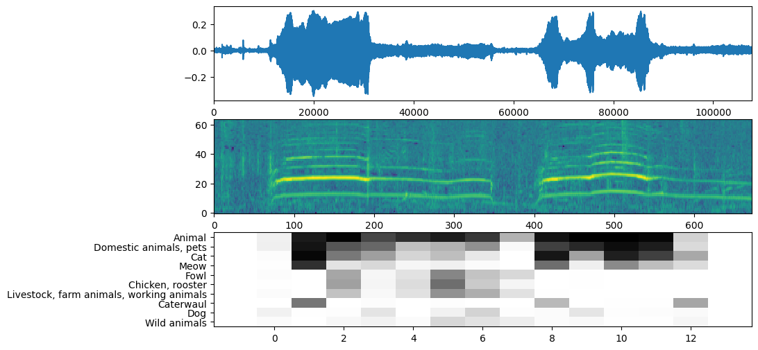
अब आसान हिस्सा: पहले से तैयार किए गए डेटा का उपयोग करके, आप बस मॉडल को कॉल करें और प्राप्त करें: स्कोर, एम्बेडिंग और स्पेक्ट्रोग्राम।
स्कोर मुख्य परिणाम है जिसका आप उपयोग करेंगे। बाद में कुछ विज़ुअलाइज़ेशन करने के लिए आप जिस स्पेक्ट्रोग्राम का उपयोग करेंगे।
# Run the model, check the output.
scores, embeddings, spectrogram = model(waveform)
scores_np = scores.numpy()
spectrogram_np = spectrogram.numpy()
infered_class = class_names[scores_np.mean(axis=0).argmax()]
print(f'The main sound is: {infered_class}')
The main sound is: Animal
VISUALIZATION
YAMNet कुछ अतिरिक्त जानकारी भी देता है जिसका उपयोग हम विज़ुअलाइज़ेशन के लिए कर सकते हैं। आइए वेवफॉर्म, स्पेक्ट्रोग्राम और अनुमानित शीर्ष वर्गों पर एक नज़र डालें।
plt.figure(figsize=(10, 6))

# Plot the waveform.
plt.subplot(3, 1, 1)
plt.plot(waveform)
plt.xlim([0, len(waveform)])

# Plot the log-mel spectrogram (returned by the model).
plt.subplot(3, 1, 2)
plt.imshow(spectrogram_np.T, aspect='auto', interpolation='nearest', origin='lower')

# Plot and label the model output scores for the top-scoring classes.
mean_scores = np.mean(scores, axis=0)
top_n = 10
top_class_indices = np.argsort(mean_scores)[::-1][:top_n]
plt.subplot(3, 1, 3)
plt.imshow(scores_np[:, top_class_indices].T, aspect='auto', interpolation='nearest', cmap='gray_r')

# patch_padding = (PATCH_WINDOW_SECONDS / 2) / PATCH_HOP_SECONDS
# values from the model documentation
patch_padding = (0.025 / 2) / 0.01
plt.xlim([-patch_padding-0.5, scores.shape[0] + patch_padding-0.5])
# Label the top_N classes.
yticks = range(0, top_n, 1)
plt.yticks(yticks, [class_names[top_class_indices[x]] for x in yticks])
_ = plt.ylim(-0.5 + np.array([top_n, 0]))