
| | |  ดูแหล่งที่มาบน GitHub ดูแหล่งที่มาบน GitHub | | |
ภาพรวม
นี้บทวิจารณ์ภาพยนตร์โน๊ตบุ๊คจัดประเภทเป็นบวกหรือลบข้อความที่ใช้ในการตรวจสอบที่ นี่คือตัวอย่างของการจัดหมวดหมู่ไบนารีชนิดที่สำคัญและใช้กันอย่างแพร่หลายของปัญหาการเรียนรู้เครื่อง
เราจะสาธิตการใช้การปรับกราฟให้เป็นมาตรฐานในสมุดบันทึกนี้โดยสร้างกราฟจากข้อมูลที่ป้อน สูตรทั่วไปสำหรับการสร้างแบบจำลองกราฟที่สร้างมาตรฐานโดยใช้เฟรมเวิร์ก Neural Structured Learning (NSL) เมื่ออินพุตไม่มีกราฟที่ชัดเจนมีดังนี้:
- สร้างการฝังสำหรับแต่ละตัวอย่างข้อความในอินพุต ซึ่งสามารถทำได้โดยใช้แบบจำลองก่อนการฝึกอบรมเช่น word2vec , หมุน , BERT ฯลฯ
- สร้างกราฟตามการฝังเหล่านี้โดยใช้เมตริกความคล้ายคลึงกัน เช่น ระยะทาง 'L2' ระยะทาง 'โคไซน์' ฯลฯ โหนดในกราฟสอดคล้องกับตัวอย่างและขอบในกราฟที่สอดคล้องกับความคล้ายคลึงกันระหว่างคู่ของตัวอย่าง
- สร้างข้อมูลการฝึกอบรมจากกราฟสังเคราะห์ด้านบนและคุณลักษณะตัวอย่าง ข้อมูลการฝึกอบรมที่ได้จะมีคุณลักษณะเพื่อนบ้านนอกเหนือจากคุณลักษณะของโหนดดั้งเดิม
- สร้างโครงข่ายประสาทเทียมเป็นโมเดลพื้นฐานโดยใช้ Keras sequential, functional หรือ subclass API
- ล้อมโมเดลพื้นฐานด้วยคลาส wrapper GraphRegularization ซึ่งจัดทำโดยเฟรมเวิร์ก NSL เพื่อสร้างโมเดล Keras กราฟใหม่ โมเดลใหม่นี้จะรวมการสูญเสียการทำให้เป็นมาตรฐานของกราฟเป็นเงื่อนไขการทำให้เป็นมาตรฐานในวัตถุประสงค์การฝึกอบรม
- ฝึกและประเมินกราฟโมเดล Keras
ความต้องการ
- ติดตั้งแพ็คเกจ Neural Structured Learning
- ติดตั้งเทนเซอร์โฟลว์ฮับ
pip install --quiet neural-structured-learningpip install --quiet tensorflow-hub
การพึ่งพาและการนำเข้า
import matplotlib.pyplot as plt
import numpy as np

import neural_structured_learning as nsl

import tensorflow as tf
import tensorflow_hub as hub

# Resets notebook state
tf.keras.backend.clear_session()

print("Version: ", tf.__version__)
print("Eager mode: ", tf.executing_eagerly())
print("Hub version: ", hub.__version__)
print(
    "GPU is",
    "available" if tf.config.list_physical_devices("GPU") else "NOT AVAILABLE")
Version:  2.8.0-rc0
Eager mode:  True
Hub version:  0.12.0
GPU is NOT AVAILABLE
2022-01-05 12:28:32.113752: E tensorflow/stream_executor/cuda/cuda_driver.cc:271] failed call to cuInit: CUDA_ERROR_NO_DEVICE: no CUDA-capable device is detected
ชุดข้อมูล IMDB
ชุดข้อมูลที่ไอเอ็ม มีข้อความ 50,000 บทวิจารณ์ภาพยนตร์จากที่ ฐานข้อมูลภาพยนตร์อินเทอร์เน็ต สิ่งเหล่านี้แบ่งออกเป็น 25,000 รีวิวสำหรับการฝึกอบรมและ 25,000 รีวิวสำหรับการทดสอบ การฝึกอบรมและการทดสอบชุดมีความสมดุลหมายถึงพวกเขามีจำนวนเท่ากับความคิดเห็นในเชิงบวกและเชิงลบ
ในบทช่วยสอนนี้ เราจะใช้ชุดข้อมูล IMDB เวอร์ชันที่ประมวลผลล่วงหน้า
ดาวน์โหลดชุดข้อมูล IMDB ที่ประมวลผลล่วงหน้า
ชุดข้อมูล IMDB มาพร้อมกับ TensorFlow มีการประมวลผลล่วงหน้าเพื่อให้บทวิจารณ์ (ลำดับของคำ) ถูกแปลงเป็นลำดับของจำนวนเต็ม โดยที่จำนวนเต็มแต่ละจำนวนจะแสดงคำเฉพาะในพจนานุกรม
รหัสต่อไปนี้ดาวน์โหลดชุดข้อมูล IMDB (หรือใช้สำเนาแคชหากดาวน์โหลดแล้ว):
imdb = tf.keras.datasets.imdb
(pp_train_data, pp_train_labels), (pp_test_data, pp_test_labels) = (
    imdb.load_data(num_words=10000))
Downloading data from https://storage.googleapis.com/tensorflow/tf-keras-datasets/imdb.npz
17465344/17464789 [==============================] - 0s 0us/step
17473536/17464789 [==============================] - 0s 0us/step
อาร์กิวเมนต์ num_words=10000 ช่วยให้ด้านบน 10,000 คำเกิดขึ้นบ่อยที่สุดในข้อมูลการฝึกอบรม คำที่หายากจะถูกละทิ้งเพื่อให้ขนาดของคำศัพท์สามารถจัดการได้
สำรวจข้อมูล
ใช้เวลาสักครู่เพื่อทำความเข้าใจรูปแบบของข้อมูล ชุดข้อมูลมีการประมวลผลล่วงหน้า แต่ละตัวอย่างคืออาร์เรย์ของจำนวนเต็มที่แสดงคำในบทวิจารณ์ภาพยนตร์ ป้ายแต่ละป้ายเป็นค่าจำนวนเต็มของ 0 หรือ 1 โดยที่ 0 คือการตรวจทานเชิงลบ และ 1 คือการตรวจทานเชิงบวก
print('Training entries: {}, labels: {}'.format(
    len(pp_train_data), len(pp_train_labels)))
training_samples_count = len(pp_train_data)
Training entries: 25000, labels: 25000
ข้อความของบทวิจารณ์ถูกแปลงเป็นจำนวนเต็ม โดยจำนวนเต็มแต่ละจำนวนจะแสดงถึงคำเฉพาะในพจนานุกรม นี่คือลักษณะของรีวิวแรก:
print(pp_train_data[0])
[1, 14, 22, 16, 43, 530, 973, 1622, 1385, 65, 458, 4468, 66, 3941, 4, 173, 36, 256, 5, 25, 100, 43, 838, 112, 50, 670, 2, 9, 35, 480, 284, 5, 150, 4, 172, 112, 167, 2, 336, 385, 39, 4, 172, 4536, 1111, 17, 546, 38, 13, 447, 4, 192, 50, 16, 6, 147, 2025, 19, 14, 22, 4, 1920, 4613, 469, 4, 22, 71, 87, 12, 16, 43, 530, 38, 76, 15, 13, 1247, 4, 22, 17, 515, 17, 12, 16, 626, 18, 2, 5, 62, 386, 12, 8, 316, 8, 106, 5, 4, 2223, 5244, 16, 480, 66, 3785, 33, 4, 130, 12, 16, 38, 619, 5, 25, 124, 51, 36, 135, 48, 25, 1415, 33, 6, 22, 12, 215, 28, 77, 52, 5, 14, 407, 16, 82, 2, 8, 4, 107, 117, 5952, 15, 256, 4, 2, 7, 3766, 5, 723, 36, 71, 43, 530, 476, 26, 400, 317, 46, 7, 4, 2, 1029, 13, 104, 88, 4, 381, 15, 297, 98, 32, 2071, 56, 26, 141, 6, 194, 7486, 18, 4, 226, 22, 21, 134, 476, 26, 480, 5, 144, 30, 5535, 18, 51, 36, 28, 224, 92, 25, 104, 4, 226, 65, 16, 38, 1334, 88, 12, 16, 283, 5, 16, 4472, 113, 103, 32, 15, 16, 5345, 19, 178, 32]
บทวิจารณ์ภาพยนตร์อาจมีความยาวต่างกัน รหัสด้านล่างแสดงจำนวนคำในการทบทวนครั้งแรกและครั้งที่สอง เนื่องจากอินพุตของโครงข่ายประสาทเทียมต้องมีความยาวเท่ากัน เราจึงต้องแก้ไขปัญหานี้ในภายหลัง
len(pp_train_data[0]), len(pp_train_data[1])
(218, 189)
แปลงจำนวนเต็มกลับเป็นคำ
อาจเป็นประโยชน์ที่จะทราบวิธีการแปลงจำนวนเต็มกลับไปเป็นข้อความที่เกี่ยวข้อง ที่นี่ เราจะสร้างฟังก์ชันตัวช่วยเพื่อสอบถามออบเจ็กต์พจนานุกรมที่มีการจับคู่จำนวนเต็มกับสตริง:
def build_reverse_word_index():
  # A dictionary mapping words to an integer index
  word_index = imdb.get_word_index()

  # The first indices are reserved
  word_index = {k: (v + 3) for k, v in word_index.items()}
  word_index['<PAD>'] = 0
  word_index['<START>'] = 1
  word_index['<UNK>'] = 2  # unknown
  word_index['<UNUSED>'] = 3
  return dict((value, key) for (key, value) in word_index.items())

reverse_word_index = build_reverse_word_index()

def decode_review(text):
  return ' '.join([reverse_word_index.get(i, '?') for i in text])
Downloading data from https://storage.googleapis.com/tensorflow/tf-keras-datasets/imdb_word_index.json
1646592/1641221 [==============================] - 0s 0us/step
1654784/1641221 [==============================] - 0s 0us/step
ตอนนี้เราสามารถใช้ decode_review ฟังก์ชั่นเพื่อแสดงข้อความสำหรับการทบทวนครั้งแรก:
decode_review(pp_train_data[0])
"<START> this film was just brilliant casting location scenery story direction everyone's really suited the part they played and you could just imagine being there robert <UNK> is an amazing actor and now the same being director <UNK> father came from the same scottish island as myself so i loved the fact there was a real connection with this film the witty remarks throughout the film were great it was just brilliant so much that i bought the film as soon as it was released for <UNK> and would recommend it to everyone to watch and the fly fishing was amazing really cried at the end it was so sad and you know what they say if you cry at a film it must have been good and this definitely was also <UNK> to the two little boy's that played the <UNK> of norman and paul they were just brilliant children are often left out of the <UNK> list i think because the stars that play them all grown up are such a big profile for the whole film but these children are amazing and should be praised for what they have done don't you think the whole story was so lovely because it was true and was someone's life after all that was shared with us all"
การสร้างกราฟ
การสร้างกราฟเกี่ยวข้องกับการสร้างการฝังสำหรับตัวอย่างข้อความ จากนั้นใช้ฟังก์ชันความคล้ายคลึงกันเพื่อเปรียบเทียบการฝัง
ก่อนดำเนินการต่อ ขั้นแรกเราจะสร้างไดเร็กทอรีเพื่อจัดเก็บอาร์ติแฟกต์ที่สร้างโดยบทช่วยสอนนี้
mkdir -p /tmp/imdb
สร้างตัวอย่างการฝัง
เราจะใช้ pretrained embeddings หมุนเพื่อสร้าง embeddings ใน tf.train.Example รูปแบบสำหรับแต่ละกลุ่มตัวอย่างในการป้อนข้อมูล เราจะเก็บ embeddings ผลใน TFRecord รูปแบบพร้อมกับคุณลักษณะเพิ่มเติมที่แสดงถึงหมายเลขของแต่ละตัวอย่าง นี่เป็นสิ่งสำคัญและจะช่วยให้เราจับคู่การฝังตัวอย่างกับโหนดที่เกี่ยวข้องในกราฟได้ในภายหลัง
pretrained_embedding = 'https://tfhub.dev/google/tf2-preview/gnews-swivel-20dim/1'

hub_layer = hub.KerasLayer(
    pretrained_embedding, input_shape=[], dtype=tf.string, trainable=True)
def _int64_feature(value):
  """Returns int64 tf.train.Feature."""
  return tf.train.Feature(int64_list=tf.train.Int64List(value=value.tolist()))


def _bytes_feature(value):
  """Returns bytes tf.train.Feature."""
  return tf.train.Feature(
      bytes_list=tf.train.BytesList(value=[value.encode('utf-8')]))


def _float_feature(value):
  """Returns float tf.train.Feature."""
  return tf.train.Feature(float_list=tf.train.FloatList(value=value.tolist()))


def create_embedding_example(word_vector, record_id):
  """Create tf.Example containing the sample's embedding and its ID."""

  text = decode_review(word_vector)

  # Shape = [batch_size,].
  sentence_embedding = hub_layer(tf.reshape(text, shape=[-1,]))

  # Flatten the sentence embedding back to 1-D.
  sentence_embedding = tf.reshape(sentence_embedding, shape=[-1])

  features = {
      'id': _bytes_feature(str(record_id)),
      'embedding': _float_feature(sentence_embedding.numpy())
  }
  return tf.train.Example(features=tf.train.Features(feature=features))


def create_embeddings(word_vectors, output_path, starting_record_id):
  record_id = int(starting_record_id)
  with tf.io.TFRecordWriter(output_path) as writer:
    for word_vector in word_vectors:
      example = create_embedding_example(word_vector, record_id)
      record_id = record_id + 1
      writer.write(example.SerializeToString())
  return record_id


# Persist TF.Example features containing embeddings for training data in
# TFRecord format.
create_embeddings(pp_train_data, '/tmp/imdb/embeddings.tfr', 0)
25000
สร้างกราฟ
ตอนนี้เรามีตัวอย่างการฝัง เราจะใช้พวกมันเพื่อสร้างกราฟความคล้ายคลึง กล่าวคือ โหนดในกราฟนี้จะสอดคล้องกับตัวอย่างและขอบในกราฟนี้จะสอดคล้องกับความคล้ายคลึงระหว่างโหนดคู่
Neural Structured Learning จัดเตรียมไลบรารีการสร้างกราฟเพื่อสร้างกราฟตามการฝังตัวอย่าง มันใช้ ความคล้ายคลึงกันโคไซน์ เป็นตัวชี้วัดความคล้ายคลึงกันเพื่อเปรียบเทียบ embeddings และสร้างขอบระหว่างพวกเขา นอกจากนี้ยังช่วยให้เราระบุเกณฑ์ความคล้ายคลึงกันได้ ซึ่งสามารถใช้เพื่อละทิ้งขอบที่ต่างไปจากกราฟสุดท้าย ในตัวอย่างนี้ โดยใช้ 0.99 เป็นเกณฑ์ความคล้ายคลึงกัน และ 12345 เป็นเมล็ดสุ่ม เราจะลงเอยด้วยกราฟที่มีขอบแบบสองทิศทาง 429,415 นี่เรากำลังใช้สนับสนุนการสร้างกราฟสำหรับ ท้องที่ที่มีความอ่อนไหวคร่ำเครียด (LSH) เพื่อเพิ่มความเร็วในการสร้างกราฟ สำหรับรายละเอียดเกี่ยวกับการใช้การสนับสนุน LSH สร้างกราฟให้ดูที่ build_graph_from_config เอกสาร API
graph_builder_config = nsl.configs.GraphBuilderConfig(
    similarity_threshold=0.99, lsh_splits=32, lsh_rounds=15, random_seed=12345)
nsl.tools.build_graph_from_config(['/tmp/imdb/embeddings.tfr'],
                                  '/tmp/imdb/graph_99.tsv',
                                  graph_builder_config)
แต่ละขอบแบบสองทิศทางจะแสดงด้วยขอบกำกับสองเส้นในไฟล์ TSV เอาต์พุต ดังนั้นไฟล์จะมี 429,415 * 2 = 858,830 บรรทัดทั้งหมด:
wc -l /tmp/imdb/graph_99.tsv
858830 /tmp/imdb/graph_99.tsv
คุณสมบัติตัวอย่าง
เราสร้างคุณลักษณะตัวอย่างสำหรับปัญหาของเราโดยใช้ tf.train.Example รูปแบบและยังคงมีอยู่พวกเขาใน TFRecord รูปแบบ แต่ละตัวอย่างจะมีคุณสมบัติสามประการต่อไปนี้:
- ID: ID โหนดของกลุ่มตัวอย่าง
- คำ: รายการ int64 มีรหัสคำ
- ป้ายชื่อ: เดี่ยว int64 ระบุระดับเป้าหมายของการตรวจสอบ
def create_example(word_vector, label, record_id):
  """Create tf.Example containing the sample's word vector, label, and ID."""
  features = {
      'id': _bytes_feature(str(record_id)),
      'words': _int64_feature(np.asarray(word_vector)),
      'label': _int64_feature(np.asarray([label])),
  }
  return tf.train.Example(features=tf.train.Features(feature=features))

def create_records(word_vectors, labels, record_path, starting_record_id):
  record_id = int(starting_record_id)
  with tf.io.TFRecordWriter(record_path) as writer:
    for word_vector, label in zip(word_vectors, labels):
      example = create_example(word_vector, label, record_id)
      record_id = record_id + 1
      writer.write(example.SerializeToString())
  return record_id

# Persist TF.Example features (word vectors and labels) for training and test
# data in TFRecord format.
next_record_id = create_records(pp_train_data, pp_train_labels,
                                '/tmp/imdb/train_data.tfr', 0)
create_records(pp_test_data, pp_test_labels, '/tmp/imdb/test_data.tfr',
               next_record_id)
50000
เพิ่มข้อมูลการฝึกอบรมด้วยกราฟเพื่อนบ้าน
เนื่องจากเรามีคุณลักษณะตัวอย่างและกราฟสังเคราะห์ เราจึงสามารถสร้างข้อมูลการฝึกอบรมเสริมสำหรับการเรียนรู้ที่มีโครงสร้างทางประสาท กรอบงาน NSL จัดให้มีห้องสมุดเพื่อรวมกราฟและคุณลักษณะตัวอย่างเพื่อสร้างข้อมูลการฝึกอบรมขั้นสุดท้ายสำหรับการปรับกราฟให้เป็นมาตรฐาน ข้อมูลการฝึกอบรมที่ได้จะรวมคุณลักษณะตัวอย่างดั้งเดิมและคุณลักษณะของเพื่อนบ้านที่เกี่ยวข้อง
ในบทช่วยสอนนี้ เราพิจารณาขอบที่ไม่มีทิศทางและใช้เพื่อนบ้านสูงสุด 3 รายการต่อตัวอย่างเพื่อเพิ่มข้อมูลการฝึกด้วยกราฟเพื่อนบ้าน
nsl.tools.pack_nbrs(
    '/tmp/imdb/train_data.tfr',
    '',
    '/tmp/imdb/graph_99.tsv',
    '/tmp/imdb/nsl_train_data.tfr',
    add_undirected_edges=True,
    max_nbrs=3)
รุ่นพื้นฐาน
ตอนนี้เราพร้อมที่จะสร้างแบบจำลองพื้นฐานโดยไม่ต้องปรับกราฟให้เป็นมาตรฐานแล้ว ในการสร้างแบบจำลองนี้ เราสามารถใช้การฝังที่ใช้ในการสร้างกราฟ หรือเรียนรู้การฝังใหม่ร่วมกับงานการจัดหมวดหมู่ สำหรับจุดประสงค์ของสมุดบันทึกนี้ เราจะทำอย่างหลัง
ตัวแปรโกลบอล
NBR_FEATURE_PREFIX = 'NL_nbr_'
NBR_WEIGHT_SUFFIX = '_weight'
ไฮเปอร์พารามิเตอร์
เราจะใช้ตัวอย่างของ HParams เพื่อ inclue hyperparameters ต่างๆและค่าคงที่ที่ใช้สำหรับการฝึกอบรมและการประเมินผล เราอธิบายโดยย่อแต่ละข้อด้านล่าง:
num_classes: มี 2 ชั้นเรียน - บวกและลบ
max_seq_length: นี่คือจำนวนสูงสุดของคำพิจารณาจากการตรวจสอบภาพยนตร์ในแต่ละตัวอย่างนี้
vocab_size: นี่คือขนาดของคำศัพท์ที่พิจารณาเช่นนี้
distance_type: นี่คือระยะทางที่ตัวชี้วัดที่ใช้ในการกฏหมายตัวอย่างกับประเทศเพื่อนบ้าน
graph_regularization_multiplier: การควบคุมนี้น้ำหนักสัมพัทธ์ของระยะกราฟกูในฟังก์ชั่นการสูญเสียโดยรวม
num_neighbors: จำนวนของประเทศเพื่อนบ้านที่ใช้สำหรับกราฟกู ค่านี้จะต้องมีค่าน้อยกว่าหรือเท่ากับ
max_nbrsอาร์กิวเมนต์สินค้าด้านบนเมื่ออัญเชิญnsl.tools.pack_nbrsnum_fc_units: จำนวนหน่วยในชั้นเชื่อมต่ออย่างเต็มที่ของเครือข่ายประสาท
train_epochs: จำนวน epochs การฝึกอบรม
ขนาดชุดที่ใช้สำหรับการฝึกอบรมและการประเมินผล: batch_size
eval_steps: จำนวนสำหรับกระบวนการที่จะดำเนินการก่อนที่จะกามารมณ์ประเมินเสร็จสมบูรณ์ หากการตั้งค่า
Noneอินสแตนซ์ทั้งหมดในชุดการทดสอบได้รับการประเมิน
class HParams(object):
  """Hyperparameters used for training."""
  def __init__(self):
    ### dataset parameters
    self.num_classes = 2
    self.max_seq_length = 256
    self.vocab_size = 10000
    ### neural graph learning parameters
    self.distance_type = nsl.configs.DistanceType.L2
    self.graph_regularization_multiplier = 0.1
    self.num_neighbors = 2
    ### model architecture
    self.num_embedding_dims = 16
    self.num_lstm_dims = 64
    self.num_fc_units = 64
    ### training parameters
    self.train_epochs = 10
    self.batch_size = 128
    ### eval parameters
    self.eval_steps = None  # All instances in the test set are evaluated.

HPARAMS = HParams()
เตรียมข้อมูล
บทวิจารณ์—อาร์เรย์ของจำนวนเต็ม—จะต้องแปลงเป็นเทนเซอร์ก่อนที่จะป้อนเข้าสู่โครงข่ายประสาทเทียม การแปลงนี้สามารถทำได้สองวิธี:
แปลงอาร์เรย์ลงในเวกเตอร์ของ
0และ1s แสดงให้เห็นการเกิดขึ้นคำคล้ายกับการเข้ารหัสร้อน ยกตัวอย่างเช่นลำดับ[3, 5]จะกลายเป็น10000เวกเตอร์มิติที่เป็นศูนย์ทั้งหมดยกเว้นดัชนี3และ5ซึ่งเป็นคน จากนั้นทำเรื่องนี้ให้ชั้นแรกในเครือข่ายของเราDenseชั้นที่สามารถจัดการกับข้อมูลจุดลอยเวกเตอร์ วิธีการนี้เป็นหน่วยความจำมาก แต่ต้องnum_words * num_reviewsขนาดเมทริกซ์หรืออีกวิธีหนึ่งที่เราสามารถแผ่นอาร์เรย์เพื่อให้พวกเขาทั้งหมดมีความยาวเดียวกันแล้วสร้างเมตริกซ์จำนวนเต็มของรูปร่าง
max_length * num_reviewsเราสามารถใช้เลเยอร์การฝังที่สามารถจัดการรูปร่างนี้เป็นเลเยอร์แรกในเครือข่ายของเรา
ในบทช่วยสอนนี้ เราจะใช้แนวทางที่สอง
ตั้งแต่บทวิจารณ์ภาพยนตร์จะต้องมีระยะเวลาเดียวกันเราจะใช้ pad_sequence ฟังก์ชั่นที่กำหนดไว้ด้านล่างเพื่อสร้างมาตรฐานความยาว
def make_dataset(file_path, training=False):
  """Creates a `tf.data.TFRecordDataset`.

  Args:
    file_path: Name of the file in the `.tfrecord` format containing
      `tf.train.Example` objects.
    training: Boolean indicating if we are in training mode.

  Returns:
    An instance of `tf.data.TFRecordDataset` containing the `tf.train.Example`
    objects.
  """

  def pad_sequence(sequence, max_seq_length):
    """Pads the input sequence (a `tf.SparseTensor`) to `max_seq_length`."""
    pad_size = tf.maximum([0], max_seq_length - tf.shape(sequence)[0])
    padded = tf.concat(
        [sequence.values,
         tf.fill((pad_size), tf.cast(0, sequence.dtype))],
        axis=0)
    # The input sequence may be larger than max_seq_length. Truncate down if
    # necessary.
    return tf.slice(padded, [0], [max_seq_length])

  def parse_example(example_proto):
    """Extracts relevant fields from the `example_proto`.

    Args:
      example_proto: An instance of `tf.train.Example`.

    Returns:
      A pair whose first value is a dictionary containing relevant features
      and whose second value contains the ground truth labels.
    """
    # The 'words' feature is a variable length word ID vector.
    feature_spec = {
        'words': tf.io.VarLenFeature(tf.int64),
        'label': tf.io.FixedLenFeature((), tf.int64, default_value=-1),
    }
    # We also extract corresponding neighbor features in a similar manner to
    # the features above during training.
    if training:
      for i in range(HPARAMS.num_neighbors):
        nbr_feature_key = '{}{}_{}'.format(NBR_FEATURE_PREFIX, i, 'words')
        nbr_weight_key = '{}{}{}'.format(NBR_FEATURE_PREFIX, i,
                                         NBR_WEIGHT_SUFFIX)
        feature_spec[nbr_feature_key] = tf.io.VarLenFeature(tf.int64)

        # We assign a default value of 0.0 for the neighbor weight so that
        # graph regularization is done on samples based on their exact number
        # of neighbors. In other words, non-existent neighbors are discounted.
        feature_spec[nbr_weight_key] = tf.io.FixedLenFeature(
            [1], tf.float32, default_value=tf.constant([0.0]))

    features = tf.io.parse_single_example(example_proto, feature_spec)

    # Since the 'words' feature is a variable length word vector, we pad it to a
    # constant maximum length based on HPARAMS.max_seq_length
    features['words'] = pad_sequence(features['words'], HPARAMS.max_seq_length)
    if training:
      for i in range(HPARAMS.num_neighbors):
        nbr_feature_key = '{}{}_{}'.format(NBR_FEATURE_PREFIX, i, 'words')
        features[nbr_feature_key] = pad_sequence(features[nbr_feature_key],
                                                 HPARAMS.max_seq_length)

    labels = features.pop('label')
    return features, labels

  dataset = tf.data.TFRecordDataset([file_path])
  if training:
    dataset = dataset.shuffle(10000)
  dataset = dataset.map(parse_example)
  dataset = dataset.batch(HPARAMS.batch_size)
  return dataset


train_dataset = make_dataset('/tmp/imdb/nsl_train_data.tfr', True)
test_dataset = make_dataset('/tmp/imdb/test_data.tfr')
สร้างแบบจำลอง
โครงข่ายประสาทเทียมถูกสร้างขึ้นโดยการซ้อนเลเยอร์ ซึ่งต้องมีการตัดสินใจทางสถาปัตยกรรมหลักสองประการ:
- ต้องใช้กี่ชั้นในโมเดล?
- วิธีการหลายหน่วยที่ซ่อนอยู่ที่จะใช้สำหรับแต่ละชั้น?
ในตัวอย่างนี้ ข้อมูลที่ป้อนเข้าประกอบด้วยอาร์เรย์ของดัชนีคำ ป้ายกำกับที่จะคาดการณ์คือ 0 หรือ 1
เราจะใช้ LSTM แบบสองทิศทางเป็นแบบจำลองพื้นฐานของเราในบทช่วยสอนนี้
# This function exists as an alternative to the bi-LSTM model used in this
# notebook.
def make_feed_forward_model():
  """Builds a simple 2 layer feed forward neural network."""
  inputs = tf.keras.Input(
      shape=(HPARAMS.max_seq_length,), dtype='int64', name='words')
  embedding_layer = tf.keras.layers.Embedding(HPARAMS.vocab_size, 16)(inputs)
  pooling_layer = tf.keras.layers.GlobalAveragePooling1D()(embedding_layer)
  dense_layer = tf.keras.layers.Dense(16, activation='relu')(pooling_layer)
  outputs = tf.keras.layers.Dense(1)(dense_layer)
  return tf.keras.Model(inputs=inputs, outputs=outputs)


def make_bilstm_model():
  """Builds a bi-directional LSTM model."""
  inputs = tf.keras.Input(
      shape=(HPARAMS.max_seq_length,), dtype='int64', name='words')
  embedding_layer = tf.keras.layers.Embedding(HPARAMS.vocab_size,
                                              HPARAMS.num_embedding_dims)(
                                                  inputs)
  lstm_layer = tf.keras.layers.Bidirectional(
      tf.keras.layers.LSTM(HPARAMS.num_lstm_dims))(
          embedding_layer)
  dense_layer = tf.keras.layers.Dense(
      HPARAMS.num_fc_units, activation='relu')(
          lstm_layer)
  outputs = tf.keras.layers.Dense(1)(dense_layer)
  return tf.keras.Model(inputs=inputs, outputs=outputs)


# Feel free to use an architecture of your choice.
model = make_bilstm_model()
model.summary()
Model: "model"
_________________________________________________________________
 Layer (type)                Output Shape              Param #
=================================================================
 words (InputLayer)          [(None, 256)]             0

 embedding (Embedding)       (None, 256, 16)           160000

 bidirectional (Bidirectiona  (None, 128)              41472
 l)

 dense (Dense)               (None, 64)                8256

 dense_1 (Dense)             (None, 1)                 65

=================================================================
Total params: 209,793
Trainable params: 209,793
Non-trainable params: 0
_________________________________________________________________
เลเยอร์ถูกซ้อนกันอย่างมีประสิทธิภาพตามลำดับเพื่อสร้างลักษณนาม:
- ชั้นแรกเป็น
Inputชั้นซึ่งจะมีคำศัพท์จำนวนเต็มเข้ารหัส - ชั้นถัดไปเป็น
Embeddingชั้นซึ่งจะมีคำศัพท์จำนวนเต็มเข้ารหัสและรูปลักษณ์ที่ขึ้นเวกเตอร์ฝังสำหรับแต่ละคำดัชนี เวกเตอร์เหล่านี้เรียนรู้เหมือนรถไฟจำลอง เวกเตอร์เพิ่มมิติให้กับอาร์เรย์เอาต์พุต ขนาดส่งผลมีดังนี้:(batch, sequence, embedding) - ถัดไป เลเยอร์ LSTM แบบสองทิศทางจะส่งกลับเวกเตอร์เอาต์พุตที่มีความยาวคงที่สำหรับแต่ละตัวอย่าง
- เวกเตอร์เอาท์พุทความยาวคงที่นี้เป็นประปาผ่านอย่างเต็มที่ที่เชื่อมต่อ (
Dense) ชั้น 64 หน่วยซ่อน - เลเยอร์สุดท้ายเชื่อมต่ออย่างหนาแน่นด้วยโหนดเอาต์พุตเดียว ใช้
sigmoidฟังก์ชั่นการเปิดใช้งานค่านี้เป็นลอยระหว่าง 0 และ 1 เป็นตัวแทนของความน่าจะเป็นหรือระดับความเชื่อมั่น
หน่วยที่ซ่อนอยู่
รูปแบบดังกล่าวข้างต้นมีสองระดับกลางหรือ "ซ่อน" ชั้นระหว่าง input และ output และไม่รวม Embedding ชั้น จำนวนเอาต์พุต (หน่วย โหนด หรือเซลล์ประสาท) คือมิติของพื้นที่แสดงแทนสำหรับเลเยอร์ กล่าวอีกนัยหนึ่ง จำนวนอิสระที่เครือข่ายได้รับอนุญาตเมื่อเรียนรู้การเป็นตัวแทนภายใน
หากโมเดลมีหน่วยที่ซ่อนอยู่มากกว่า (พื้นที่การแสดงในมิติที่สูงกว่า) และ/หรือเลเยอร์มากกว่า เครือข่ายก็สามารถเรียนรู้การแทนค่าที่ซับซ้อนมากขึ้นได้ อย่างไรก็ตาม มันทำให้เครือข่ายมีค่าใช้จ่ายในการคำนวณมากขึ้น และอาจนำไปสู่การเรียนรู้รูปแบบที่ไม่ต้องการ—รูปแบบที่ปรับปรุงประสิทธิภาพในข้อมูลการฝึกแต่ไม่ใช่ในข้อมูลการทดสอบ นี้เรียกว่าอิง
ฟังก์ชั่นการสูญเสียและเครื่องมือเพิ่มประสิทธิภาพ
โมเดลต้องมีฟังก์ชันการสูญเสียและเครื่องมือเพิ่มประสิทธิภาพสำหรับการฝึกอบรม ตั้งแต่นี้เป็นปัญหาที่จำแนกไบนารีและรูปแบบความน่าจะเป็นเอาท์พุท (ชั้นหน่วยเดียวที่มีการเปิดใช้งาน sigmoid) เราจะใช้ binary_crossentropy ฟังก์ชั่นการสูญเสีย
model.compile(
    optimizer='adam',
    loss=tf.keras.losses.BinaryCrossentropy(from_logits=True),
    metrics=['accuracy'])
สร้างชุดการตรวจสอบ
เมื่อทำการฝึกอบรม เราต้องการตรวจสอบความถูกต้องของแบบจำลองกับข้อมูลที่ไม่เคยเห็นมาก่อน สร้างชุดการตรวจสอบโดยการตั้งค่าออกจากกันส่วนของข้อมูลการฝึกอบรมเดิม (ทำไมไม่ใช้ชุดการทดสอบตอนนี้ล่ะ เป้าหมายของเราคือการพัฒนาและปรับแต่งแบบจำลองของเราโดยใช้ข้อมูลการฝึกอบรมเท่านั้น จากนั้นใช้ข้อมูลการทดสอบเพียงครั้งเดียวเพื่อประเมินความถูกต้องของเรา)
ในบทช่วยสอนนี้ เรานำตัวอย่างการฝึกเริ่มต้นประมาณ 10% (10% จาก 25000) เป็นข้อมูลที่มีป้ายกำกับสำหรับการฝึกอบรม และส่วนที่เหลือเป็นข้อมูลการตรวจสอบ เนื่องจากการแบ่งรถไฟ/การทดสอบเริ่มต้นคือ 50/50 (แต่ละตัวอย่าง 25,000 ตัวอย่าง) การแยกการฝึก/การตรวจสอบ/การทดสอบที่มีประสิทธิภาพตอนนี้ที่เรามีคือ 5/45/50
โปรดทราบว่า 'train_dataset' ได้รับแบทช์และสับเปลี่ยนแล้ว
validation_fraction = 0.9
validation_size = int(validation_fraction *
                      int(training_samples_count / HPARAMS.batch_size))
print(validation_size)
validation_dataset = train_dataset.take(validation_size)
train_dataset = train_dataset.skip(validation_size)
175
ฝึกโมเดล
ฝึกโมเดลในมินิแบตช์ ขณะฝึก ให้ตรวจสอบการสูญเสียและความแม่นยำของแบบจำลองในชุดตรวจสอบความถูกต้อง:
history = model.fit(
    train_dataset,
    validation_data=validation_dataset,
    epochs=HPARAMS.train_epochs,
    verbose=1)
Epoch 1/10
/tmpfs/src/tf_docs_env/lib/python3.7/site-packages/keras/engine/functional.py:559: UserWarning: Input dict contained keys ['NL_nbr_0_words', 'NL_nbr_1_words', 'NL_nbr_0_weight', 'NL_nbr_1_weight'] which did not match any model input. They will be ignored by the model.
  inputs = self._flatten_to_reference_inputs(inputs)
21/21 [==============================] - 22s 889ms/step - loss: 0.6932 - accuracy: 0.5065 - val_loss: 0.6928 - val_accuracy: 0.5004
Epoch 2/10
21/21 [==============================] - 17s 841ms/step - loss: 0.6918 - accuracy: 0.5000 - val_loss: 0.6843 - val_accuracy: 0.4988
Epoch 3/10
21/21 [==============================] - 17s 839ms/step - loss: 0.6677 - accuracy: 0.5069 - val_loss: 0.5976 - val_accuracy: 0.6507
Epoch 4/10
21/21 [==============================] - 17s 836ms/step - loss: 0.5579 - accuracy: 0.6912 - val_loss: 0.4801 - val_accuracy: 0.7974
Epoch 5/10
21/21 [==============================] - 17s 837ms/step - loss: 0.4377 - accuracy: 0.7965 - val_loss: 0.3678 - val_accuracy: 0.8372
Epoch 6/10
21/21 [==============================] - 17s 836ms/step - loss: 0.3526 - accuracy: 0.8408 - val_loss: 0.4261 - val_accuracy: 0.8283
Epoch 7/10
21/21 [==============================] - 17s 835ms/step - loss: 0.4090 - accuracy: 0.8273 - val_loss: 0.3961 - val_accuracy: 0.8346
Epoch 8/10
21/21 [==============================] - 17s 834ms/step - loss: 0.3105 - accuracy: 0.8842 - val_loss: 0.2976 - val_accuracy: 0.8813
Epoch 9/10
21/21 [==============================] - 17s 834ms/step - loss: 0.3335 - accuracy: 0.8673 - val_loss: 0.3373 - val_accuracy: 0.8537
Epoch 10/10
21/21 [==============================] - 17s 837ms/step - loss: 0.3104 - accuracy: 0.8765 - val_loss: 0.2804 - val_accuracy: 0.8902
ประเมินแบบจำลอง
ตอนนี้เรามาดูกันว่าโมเดลทำงานอย่างไร สองค่าจะถูกส่งกลับ การสูญเสีย (ตัวเลขที่แสดงถึงข้อผิดพลาดของเรา ค่าที่ต่ำกว่าจะดีกว่า) และความแม่นยำ
results = model.evaluate(test_dataset, steps=HPARAMS.eval_steps)
print(results)
196/196 [==============================] - 16s 76ms/step - loss: 0.3695 - accuracy: 0.8389
[0.3694916367530823, 0.838919997215271]
สร้างกราฟความแม่นยำ/การสูญเสียเมื่อเวลาผ่านไป
model.fit() ส่งกลับ History วัตถุที่มีพจนานุกรมกับทุกสิ่งที่เกิดขึ้นในระหว่างการฝึก:
history_dict = history.history
history_dict.keys()
dict_keys(['loss', 'accuracy', 'val_loss', 'val_accuracy'])
มีสี่รายการ: หนึ่งรายการสำหรับแต่ละเมตริกที่ถูกตรวจสอบระหว่างการฝึกอบรมและการตรวจสอบ เราสามารถใช้สิ่งเหล่านี้เพื่อวางแผนการสูญเสียการฝึกอบรมและการตรวจสอบเพื่อการเปรียบเทียบ รวมถึงความแม่นยำของการฝึกอบรมและการตรวจสอบ:
acc = history_dict['accuracy']
val_acc = history_dict['val_accuracy']
loss = history_dict['loss']
val_loss = history_dict['val_loss']
epochs = range(1, len(acc) + 1)
# "-r^" is for solid red line with triangle markers.
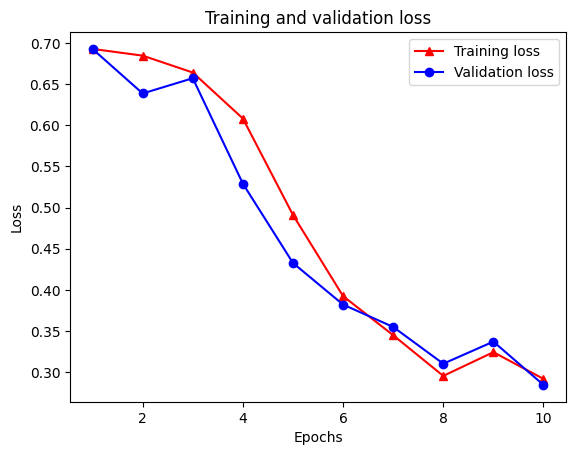
plt.plot(epochs, loss, '-r^', label='Training loss')
# "-b0" is for solid blue line with circle markers.
plt.plot(epochs, val_loss, '-bo', label='Validation loss')
plt.title('Training and validation loss')
plt.xlabel('Epochs')
plt.ylabel('Loss')
plt.legend(loc='best')
plt.show()
plt.clf()   # clear figure

plt.plot(epochs, acc, '-r^', label='Training acc')
plt.plot(epochs, val_acc, '-bo', label='Validation acc')
plt.title('Training and validation accuracy')
plt.xlabel('Epochs')
plt.ylabel('Accuracy')
plt.legend(loc='best')

plt.show()
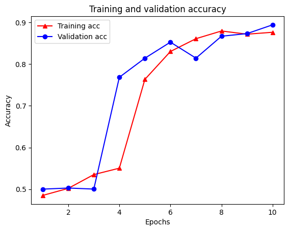
ขอให้สังเกตการฝึกอบรมการสูญเสียลดลงด้วยในแต่ละยุคและการเพิ่มขึ้นของความถูกต้องของการฝึกอบรมกับแต่ละยุค สิ่งนี้คาดหวังเมื่อใช้การเพิ่มประสิทธิภาพการไล่ระดับการไล่ระดับสี—ควรลดปริมาณที่ต้องการให้น้อยที่สุดในการวนซ้ำทุกครั้ง
การทำให้เป็นมาตรฐานของกราฟ
ตอนนี้เราพร้อมที่จะลองใช้การปรับกราฟให้เป็นมาตรฐานโดยใช้โมเดลพื้นฐานที่เราสร้างไว้ด้านบน เราจะใช้ GraphRegularization ชั้นเสื้อคลุมให้โดยกรอบการเรียนรู้ประสาทโครงสร้างการห่อฐาน (สอง LSTM) รุ่นที่จะรวมถึงกูกราฟ ขั้นตอนที่เหลือสำหรับการฝึกและประเมินแบบจำลองที่สร้างกราฟจะคล้ายกับขั้นตอนของแบบจำลองพื้นฐาน
สร้างแบบจำลองกราฟปกติ
ในการประเมินประโยชน์ที่เพิ่มขึ้นของการทำให้กราฟเป็นมาตรฐาน เราจะสร้างอินสแตนซ์โมเดลพื้นฐานใหม่ เพราะนี่คือ model ได้รับการฝึกไม่กี่ซ้ำและการนำรูปแบบการฝึกอบรมนี้เพื่อสร้างรูปแบบกราฟ regularized จะไม่เปรียบเทียบยุติธรรมสำหรับ model
# Build a new base LSTM model.
base_reg_model = make_bilstm_model()
# Wrap the base model with graph regularization.
graph_reg_config = nsl.configs.make_graph_reg_config(
    max_neighbors=HPARAMS.num_neighbors,
    multiplier=HPARAMS.graph_regularization_multiplier,
    distance_type=HPARAMS.distance_type,
    sum_over_axis=-1)
graph_reg_model = nsl.keras.GraphRegularization(base_reg_model,
                                                graph_reg_config)
graph_reg_model.compile(
    optimizer='adam',
    loss=tf.keras.losses.BinaryCrossentropy(from_logits=True),
    metrics=['accuracy'])
ฝึกโมเดล
graph_reg_history = graph_reg_model.fit(
    train_dataset,
    validation_data=validation_dataset,
    epochs=HPARAMS.train_epochs,
    verbose=1)
Epoch 1/10
/tmpfs/src/tf_docs_env/lib/python3.7/site-packages/tensorflow/python/framework/indexed_slices.py:446: UserWarning: Converting sparse IndexedSlices(IndexedSlices(indices=Tensor("gradient_tape/GraphRegularization/graph_loss/Reshape_1:0", shape=(None,), dtype=int32), values=Tensor("gradient_tape/GraphRegularization/graph_loss/Reshape:0", shape=(None, 1), dtype=float32), dense_shape=Tensor("gradient_tape/GraphRegularization/graph_loss/Cast:0", shape=(2,), dtype=int32))) to a dense Tensor of unknown shape. This may consume a large amount of memory.
  "shape. This may consume a large amount of memory." % value)
21/21 [==============================] - 28s 1s/step - loss: 0.6928 - accuracy: 0.5131 - scaled_graph_loss: 4.3840e-05 - val_loss: 0.6923 - val_accuracy: 0.4997
Epoch 2/10
21/21 [==============================] - 19s 939ms/step - loss: 0.6852 - accuracy: 0.5158 - scaled_graph_loss: 0.0021 - val_loss: 0.6818 - val_accuracy: 0.4996
Epoch 3/10
21/21 [==============================] - 19s 939ms/step - loss: 0.6698 - accuracy: 0.5123 - scaled_graph_loss: 0.0021 - val_loss: 0.6534 - val_accuracy: 0.5001
Epoch 4/10
21/21 [==============================] - 20s 959ms/step - loss: 0.6194 - accuracy: 0.6285 - scaled_graph_loss: 0.0284 - val_loss: 0.5297 - val_accuracy: 0.7955
Epoch 5/10
21/21 [==============================] - 19s 937ms/step - loss: 0.5805 - accuracy: 0.7346 - scaled_graph_loss: 0.0545 - val_loss: 0.5601 - val_accuracy: 0.6349
Epoch 6/10
21/21 [==============================] - 19s 934ms/step - loss: 0.5509 - accuracy: 0.7662 - scaled_graph_loss: 0.0654 - val_loss: 0.4899 - val_accuracy: 0.7538
Epoch 7/10
21/21 [==============================] - 19s 937ms/step - loss: 0.5326 - accuracy: 0.7877 - scaled_graph_loss: 0.0701 - val_loss: 0.4395 - val_accuracy: 0.7923
Epoch 8/10
21/21 [==============================] - 20s 940ms/step - loss: 0.5157 - accuracy: 0.8258 - scaled_graph_loss: 0.0811 - val_loss: 0.4585 - val_accuracy: 0.7909
Epoch 9/10
21/21 [==============================] - 19s 937ms/step - loss: 0.5063 - accuracy: 0.8388 - scaled_graph_loss: 0.0868 - val_loss: 0.4272 - val_accuracy: 0.8433
Epoch 10/10
21/21 [==============================] - 19s 934ms/step - loss: 0.5053 - accuracy: 0.8438 - scaled_graph_loss: 0.0858 - val_loss: 0.4485 - val_accuracy: 0.7680
ประเมินแบบจำลอง
graph_reg_results = graph_reg_model.evaluate(test_dataset, steps=HPARAMS.eval_steps)
print(graph_reg_results)
196/196 [==============================] - 16s 76ms/step - loss: 0.4890 - accuracy: 0.7246
[0.4889770448207855, 0.7246000170707703]
สร้างกราฟความแม่นยำ/การสูญเสียเมื่อเวลาผ่านไป
graph_reg_history_dict = graph_reg_history.history
graph_reg_history_dict.keys()
dict_keys(['loss', 'accuracy', 'scaled_graph_loss', 'val_loss', 'val_accuracy'])
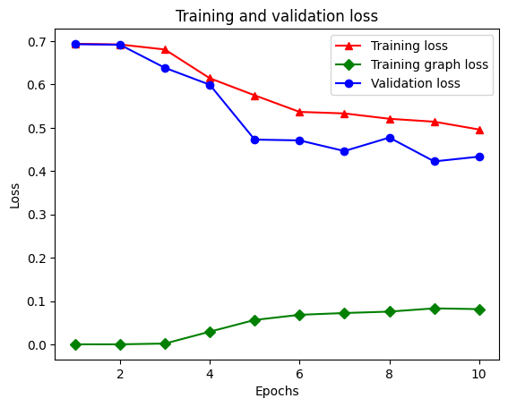
มีทั้งหมดห้ารายการในพจนานุกรม: การสูญเสียการฝึกอบรม ความแม่นยำการฝึกอบรม การสูญเสียกราฟการฝึกอบรม การสูญเสียการตรวจสอบ และความถูกต้องในการตรวจสอบ เราสามารถพล็อตมันทั้งหมดเข้าด้วยกันเพื่อเปรียบเทียบ โปรดทราบว่าการสูญเสียกราฟจะคำนวณระหว่างการฝึกเท่านั้น
acc = graph_reg_history_dict['accuracy']
val_acc = graph_reg_history_dict['val_accuracy']
loss = graph_reg_history_dict['loss']
graph_loss = graph_reg_history_dict['scaled_graph_loss']
val_loss = graph_reg_history_dict['val_loss']

epochs = range(1, len(acc) + 1)

plt.clf()   # clear figure

# "-r^" is for solid red line with triangle markers.
plt.plot(epochs, loss, '-r^', label='Training loss')
# "-gD" is for solid green line with diamond markers.
plt.plot(epochs, graph_loss, '-gD', label='Training graph loss')
# "-b0" is for solid blue line with circle markers.
plt.plot(epochs, val_loss, '-bo', label='Validation loss')
plt.title('Training and validation loss')
plt.xlabel('Epochs')
plt.ylabel('Loss')
plt.legend(loc='best')

plt.show()
plt.clf() # clear figure
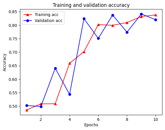
plt.plot(epochs, acc, '-r^', label='Training acc')
plt.plot(epochs, val_acc, '-bo', label='Validation acc')
plt.title('Training and validation accuracy')
plt.xlabel('Epochs')
plt.ylabel('Accuracy')
plt.legend(loc='best')
plt.show()
พลังของการเรียนรู้กึ่งควบคุม
การเรียนรู้แบบกึ่งควบคุมดูแลและโดยเฉพาะอย่างยิ่ง การปรับกราฟให้เป็นมาตรฐานในบริบทของบทช่วยสอนนี้อาจมีประสิทธิภาพมากเมื่อมีข้อมูลการฝึกอบรมเพียงเล็กน้อย การขาดข้อมูลการฝึกอบรมได้รับการชดเชยโดยใช้ประโยชน์จากความคล้ายคลึงกันระหว่างตัวอย่างการฝึกอบรม ซึ่งไม่สามารถทำได้ในการเรียนรู้ภายใต้การดูแลแบบเดิม
เรากำหนดอัตราส่วนการกำกับดูแลเป็นอัตราส่วนของตัวอย่างการฝึกอบรมเพื่อจำนวนของกลุ่มตัวอย่างซึ่งรวมถึงตัวอย่างการฝึกอบรมการตรวจสอบและทดสอบ ในสมุดบันทึกนี้ เราใช้อัตราส่วนการดูแลที่ 0.05 (กล่าวคือ 5% ของข้อมูลที่ติดป้ายกำกับ) สำหรับการฝึกทั้งรุ่นพื้นฐานและแบบจำลองที่สร้างกราฟ เราแสดงให้เห็นผลกระทบของอัตราส่วนการควบคุมดูแลต่อความแม่นยำของแบบจำลองในเซลล์ด้านล่าง
# Accuracy values for both the Bi-LSTM model and the feed forward NN model have
# been precomputed for the following supervision ratios.

supervision_ratios = [0.3, 0.15, 0.05, 0.03, 0.02, 0.01, 0.005]

model_tags = ['Bi-LSTM model', 'Feed Forward NN model']
base_model_accs = [[84, 84, 83, 80, 65, 52, 50], [87, 86, 76, 74, 67, 52, 51]]
graph_reg_model_accs = [[84, 84, 83, 83, 65, 63, 50],
                        [87, 86, 80, 75, 67, 52, 50]]

plt.clf()  # clear figure

fig, axes = plt.subplots(1, 2)
fig.set_size_inches((12, 5))

for ax, model_tag, base_model_acc, graph_reg_model_acc in zip(
    axes, model_tags, base_model_accs, graph_reg_model_accs):

  # "-r^" is for solid red line with triangle markers.
  ax.plot(base_model_acc, '-r^', label='Base model')
  # "-gD" is for solid green line with diamond markers.
  ax.plot(graph_reg_model_acc, '-gD', label='Graph-regularized model')
  ax.set_title(model_tag)
  ax.set_xlabel('Supervision ratio')
  ax.set_ylabel('Accuracy(%)')
  ax.set_ylim((25, 100))
  ax.set_xticks(range(len(supervision_ratios)))
  ax.set_xticklabels(supervision_ratios)
  ax.legend(loc='best')

plt.show()
<Figure size 432x288 with 0 Axes>
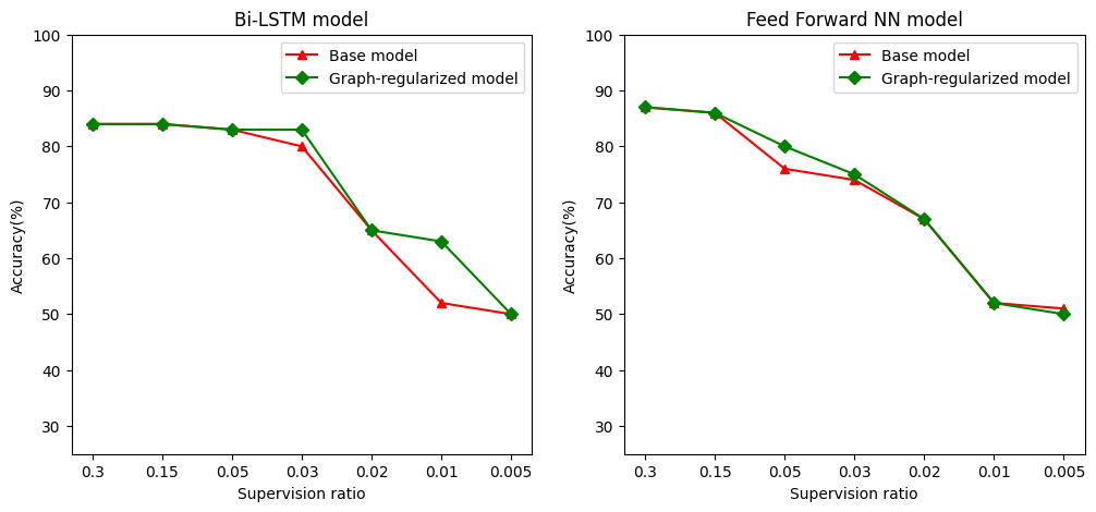
สามารถสังเกตได้ว่าเมื่ออัตราส่วนการกำกับดูแลลดลง ความแม่นยำของแบบจำลองก็ลดลงด้วย สิ่งนี้เป็นจริงสำหรับทั้งโมเดลพื้นฐานและสำหรับโมเดลที่ปรับกราฟ โดยไม่คำนึงถึงสถาปัตยกรรมของโมเดลที่ใช้ อย่างไรก็ตาม โปรดสังเกตว่าโมเดลที่สร้างกราฟให้เป็นมาตรฐานนั้นทำงานได้ดีกว่าโมเดลพื้นฐานสำหรับสถาปัตยกรรมทั้งสอง โดยเฉพาะอย่างยิ่งสำหรับรูปแบบ Bi-LSTM เมื่ออัตราส่วนการกำกับดูแลคือ 0.01 ความถูกต้องของรูปแบบกราฟ regularized เป็น ~ 20% สูงกว่าที่ฐานแบบจำลอง สาเหตุหลักมาจากการเรียนรู้กึ่งควบคุมสำหรับโมเดลที่สร้างกราฟแบบปกติ ซึ่งมีความคล้ายคลึงกันทางโครงสร้างระหว่างตัวอย่างการฝึก นอกเหนือไปจากตัวอย่างการฝึกด้วยตัวมันเอง
บทสรุป
เราได้สาธิตการใช้กราฟการทำให้เป็นมาตรฐานโดยใช้เฟรมเวิร์ก Neural Structured Learning (NSL) แม้ว่าอินพุตจะไม่มีกราฟที่ชัดเจนก็ตาม เราพิจารณางานการจัดหมวดหมู่ความเห็นของบทวิจารณ์ภาพยนตร์ IMDB ซึ่งเราสังเคราะห์กราฟความคล้ายคลึงตามการฝังบทวิจารณ์ เราสนับสนุนให้ผู้ใช้ทำการทดลองเพิ่มเติมด้วยไฮเปอร์พารามิเตอร์ที่แตกต่างกัน ปริมาณการควบคุมดูแล และโดยการใช้สถาปัตยกรรมแบบจำลองที่แตกต่างกัน