هدف این نوتبوک این است که به TFP 0.13.0 کمک کند تا از طریق چند قطعه کوچک زنده شود - دموهای کوچکی از چیزهایی که میتوانید با TFP به دست آورید.
| | |  مشاهده منبع در GitHub مشاهده منبع در GitHub | |
نصب و واردات
!pip3 install -qU tensorflow==2.5.0 tensorflow_probability==0.13.0 tensorflow-datasets inference_gym

import tensorflow as tf
import tensorflow_probability as tfp
assert '0.13' in tfp.__version__, tfp.__version__
assert '2.5' in tf.__version__, tf.__version__

physical_devices = tf.config.list_physical_devices('CPU')
tf.config.set_logical_device_configuration(
    physical_devices[0],
    [tf.config.LogicalDeviceConfiguration(),
     tf.config.LogicalDeviceConfiguration()])

tfd = tfp.distributions
tfb = tfp.bijectors
tfpk = tfp.math.psd_kernels

import matplotlib.pyplot as plt
import numpy as np
import scipy.interpolate
import IPython
import seaborn as sns
import logging
[K     |████████████████████████████████| 5.4MB 8.8MB/s
[K     |████████████████████████████████| 3.9MB 37.1MB/s
[K     |████████████████████████████████| 296kB 31.6MB/s
[?25h
توزیع ها [ریاضی هسته ای]
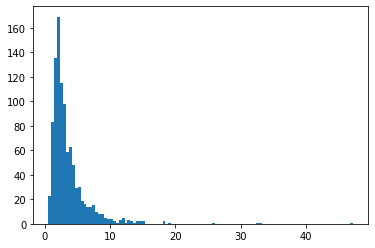
BetaQuotient
نسبت دو متغیر تصادفی مستقل با توزیع بتا
plt.hist(tfd.BetaQuotient(concentration1_numerator=5.,
                          concentration0_numerator=2.,
                          concentration1_denominator=3.,
                          concentration0_denominator=8.).sample(1_000, seed=(1, 23)),
         bins='auto');
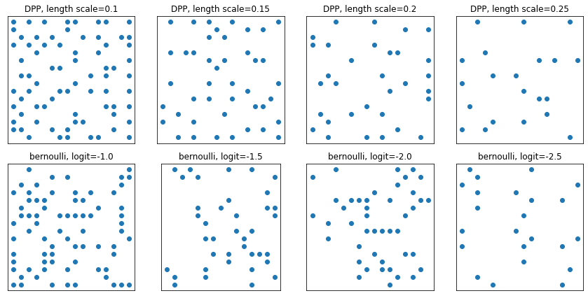
DeterminantalPointProcess
توزیع بر روی زیر مجموعهها (که به صورت یک داغ نشان داده میشود) یک مجموعه معین. نمونه ها از خاصیت دافعه پیروی می کنند (احتمالات متناسب با حجم بردارهای مربوط به زیرمجموعه انتخاب شده از نقاط است)، که به سمت نمونه گیری از زیر مجموعه های متنوع تمایل دارد. [مقایسه با نمونه iid برنولی.]
grid_size = 16
# Generate grid_size**2 pts on the unit square.
grid = np.arange(0, 1, 1./grid_size).astype(np.float32)
import itertools
points = np.array(list(itertools.product(grid, grid)))

# Create the kernel L that parameterizes the DPP.
kernel_amplitude = 2.
kernel_lengthscale = [.1, .15, .2, .25]  # Increasing length scale indicates more points are "nearby", tending toward smaller subsets.
kernel = tfpk.ExponentiatedQuadratic(kernel_amplitude, kernel_lengthscale)
kernel_matrix = kernel.matrix(points, points)

eigenvalues, eigenvectors = tf.linalg.eigh(kernel_matrix)
dpp = tfd.DeterminantalPointProcess(eigenvalues, eigenvectors)
print(dpp)

# The inner-most dimension of the result of `dpp.sample` is a multi-hot
# encoding of a subset of {1, ..., ground_set_size}.
# We will compare against a bernoulli distribution.
samps_dpp = dpp.sample(seed=(1, 2))  # 4 x grid_size**2
logits = tf.broadcast_to([[-1.], [-1.5], [-2], [-2.5]], [4, grid_size**2])
samps_bern = tfd.Bernoulli(logits=logits).sample(seed=(2, 3))

plt.figure(figsize=(12, 6))
for i, (samp, samp_bern) in enumerate(zip(samps_dpp, samps_bern)):
  plt.subplot(241 + i)
  plt.scatter(*points[np.where(samp)].T)
  plt.title(f'DPP, length scale={kernel_lengthscale[i]}')
  plt.xticks([])
  plt.yticks([])
  plt.gca().set_aspect(1.)
  plt.subplot(241 + i + 4)
  plt.scatter(*points[np.where(samp_bern)].T)
  plt.title(f'bernoulli, logit={logits[i,0]}')
  plt.xticks([])
  plt.yticks([])
  plt.gca().set_aspect(1.)

plt.tight_layout()
plt.show()
tfp.distributions.DeterminantalPointProcess("DeterminantalPointProcess", batch_shape=[4], event_shape=[256], dtype=int32)
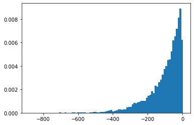
SigmoidBeta
شانس ورود دو توزیع گاما. بیشتر عددی فضای نمونه با ثبات تر از Beta .
plt.hist(tfd.SigmoidBeta(concentration1=.01, concentration0=2.).sample(10_000, seed=(1, 23)),
         bins='auto', density=True);
plt.show()

print('Old way, fractions non-finite:')
print(np.sum(~tf.math.is_finite(
    tfb.Invert(tfb.Sigmoid())(tfd.Beta(concentration1=.01, concentration0=2.)).sample(10_000, seed=(1, 23)))) / 10_000)
print(np.sum(~tf.math.is_finite(
    tfb.Invert(tfb.Sigmoid())(tfd.Beta(concentration1=2., concentration0=.01)).sample(10_000, seed=(2, 34)))) / 10_000)
Old way, fractions non-finite:
0.4215
0.8624
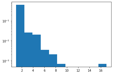
Zipf
پشتیبانی JAX اضافه شد.
plt.hist(tfd.Zipf(3.).sample(1_000, seed=(12, 34)).numpy(), bins='auto', density=True, log=True);
NormalInverseGaussian
خانواده پارامتریک انعطاف پذیر که از دم های سنگین، کج و وانیلی نرمال پشتیبانی می کند.
MatrixNormalLinearOperator
توزیع نرمال ماتریس
# Initialize a single 2 x 3 Matrix Normal.
mu = [[1., 2, 3], [3., 4, 5]]
col_cov = [[ 0.36,  0.12,  0.06],
           [ 0.12,  0.29, -0.13],
           [ 0.06, -0.13,  0.26]]
scale_column = tf.linalg.LinearOperatorLowerTriangular(tf.linalg.cholesky(col_cov))
scale_row = tf.linalg.LinearOperatorDiag([0.9, 0.8])

mvn = tfd.MatrixNormalLinearOperator(loc=mu, scale_row=scale_row, scale_column=scale_column)
mvn.sample()
WARNING:tensorflow:From /usr/local/lib/python3.7/dist-packages/tensorflow/python/ops/linalg/linear_operator_kronecker.py:224: LinearOperator.graph_parents (from tensorflow.python.ops.linalg.linear_operator) is deprecated and will be removed in a future version.
Instructions for updating:
Do not call `graph_parents`.
<tf.Tensor: shape=(2, 3), dtype=float32, numpy=
array([[1.2495145, 1.549366 , 3.2748342],
       [3.7330258, 4.3413105, 4.83423  ]], dtype=float32)>
MatrixStudentTLinearOperator
توزیع ماتریس T.
mu = [[1., 2, 3], [3., 4, 5]]
col_cov = [[ 0.36,  0.12,  0.06],
           [ 0.12,  0.29, -0.13],
           [ 0.06, -0.13,  0.26]]
scale_column = tf.linalg.LinearOperatorLowerTriangular(tf.linalg.cholesky(col_cov))
scale_row = tf.linalg.LinearOperatorDiag([0.9, 0.8])

mvn = tfd.MatrixTLinearOperator(
    df=2.,
    loc=mu,
    scale_row=scale_row,
    scale_column=scale_column)
mvn.sample()
<tf.Tensor: shape=(2, 3), dtype=float32, numpy=
array([[1.6549466, 2.6708362, 2.8629923],
       [2.1222284, 3.6904747, 5.08014  ]], dtype=float32)>
توزیع ها [نرم افزار / بسته بندی]
Sharded
بخشهای رویداد مستقل یک توزیع را در چندین پردازنده تقسیم میکند. مصالح log_prob در سراسر دستگاه، دستگیره شیب در کنسرت با tfp.experimental.distribute.JointDistribution* . زیادی را در بیشتر استنتاج توزیع نوت بوک.
strategy = tf.distribute.MirroredStrategy()

@tf.function
def sample_and_lp(seed):
  d = tfp.experimental.distribute.Sharded(tfd.Normal(0, 1))
  s = d.sample(seed=seed)
  return s, d.log_prob(s)

strategy.run(sample_and_lp, args=(tf.constant([12,34]),))
WARNING:tensorflow:There are non-GPU devices in `tf.distribute.Strategy`, not using nccl allreduce.
WARNING:tensorflow:Collective ops is not configured at program startup. Some performance features may not be enabled.
INFO:tensorflow:Using MirroredStrategy with devices ('/job:localhost/replica:0/task:0/device:CPU:0', '/job:localhost/replica:0/task:0/device:CPU:1')
INFO:tensorflow:Reduce to /job:localhost/replica:0/task:0/device:CPU:0 then broadcast to ('/job:localhost/replica:0/task:0/device:CPU:0', '/job:localhost/replica:0/task:0/device:CPU:1').
(PerReplica:{
   0: <tf.Tensor: shape=(), dtype=float32, numpy=0.0051413667>,
   1: <tf.Tensor: shape=(), dtype=float32, numpy=-0.3393052>
 }, PerReplica:{
   0: <tf.Tensor: shape=(), dtype=float32, numpy=-1.8954543>,
   1: <tf.Tensor: shape=(), dtype=float32, numpy=-1.8954543>
 })
BatchBroadcast
به طور ضمنی با یا به یک شکل دسته ای داده پخش ابعاد دسته ای از یک توزیع زمینه ای است.
underlying = tfd.MultivariateNormalDiag(tf.zeros([7, 1, 5]), tf.ones([5]))
print('underlying:', underlying)

d = tfd.BatchBroadcast(underlying, [8, 1, 6])
print('broadcast [7, 1] *with* [8, 1, 6]:', d)

try:
  tfd.BatchBroadcast(underlying, to_shape=[8, 1, 6])
except ValueError as e:
  print('broadcast [7, 1] *to* [8, 1, 6] is invalid:', e)

d = tfd.BatchBroadcast(underlying, to_shape=[8, 7, 6])
print('broadcast [7, 1] *to* [8, 7, 6]:', d)
underlying: tfp.distributions.MultivariateNormalDiag("MultivariateNormalDiag", batch_shape=[7, 1], event_shape=[5], dtype=float32)
broadcast [7, 1] *with* [8, 1, 6]: tfp.distributions.BatchBroadcast("BatchBroadcastMultivariateNormalDiag", batch_shape=[8, 7, 6], event_shape=[5], dtype=float32)
broadcast [7, 1] *to* [8, 1, 6] is invalid: Argument `to_shape` ([8 1 6]) is incompatible with underlying distribution batch shape ((7, 1)).
broadcast [7, 1] *to* [8, 7, 6]: tfp.distributions.BatchBroadcast("BatchBroadcastMultivariateNormalDiag", batch_shape=[8, 7, 6], event_shape=[5], dtype=float32)
Masked
برای تک برنامه / چند داده ها و یا پراکنده به عنوان پوشانده متراکم استفاده از موارد، یک توزیع که ماسک از log_prob از توزیعهای زمینه نامعتبر است.
d = tfd.Masked(tfd.Normal(tf.zeros([7]), 1),
               validity_mask=tf.sequence_mask([3, 4], 7))
print(d.log_prob(d.sample(seed=(1, 1))))

d = tfd.Masked(tfd.Normal(0, 1),
               validity_mask=[False, True, False],
               safe_sample_fn=tfd.Distribution.mode)
print(d.log_prob(d.sample(seed=(2, 2))))
tf.Tensor(
[[-2.3054113 -1.8524303 -1.2220721  0.         0.         0.

   0.       ]
 [-1.118623  -1.1370811 -1.1574132 -5.884986   0.         0.
   0.       ]], shape=(2, 7), dtype=float32)
tf.Tensor([ 0.         -0.93683904  0.        ], shape=(3,), dtype=float32)
بیژکتورها
- بیژکتورها
- اضافه کردن bijectors به تقلید
tf.nest.flatten(tfb.tree_flatten) وtf.nest.pack_sequence_as(tfb.pack_sequence_as). - می افزاید
tfp.experimental.bijectors.Sharded - حذف بد دانسته
tfb.ScaleTrilL. استفاده ازtfb.FillScaleTriLبه جای. - می افزاید
cls.parameter_properties()حاشیه نویسی برای Bijectors. - گسترش دامنه
tfb.Powerبه همه اعداد حقیقی برای قدرت های عدد صحیح فرد. - log-deg-jacobian بیژکتورهای اسکالر را با استفاده از autodiff استنباط کنید، در صورتی که غیر از این مشخص نشده باشد.
- اضافه کردن bijectors به تقلید
بازسازی بیژکتورها
ex = (tf.constant(1.), dict(b=tf.constant(2.), c=tf.constant(3.)))
b = tfb.tree_flatten(ex)
print(b.forward(ex))
print(b.inverse(list(tf.constant([1., 2, 3]))))

b = tfb.pack_sequence_as(ex)
print(b.forward(list(tf.constant([1., 2, 3]))))
print(b.inverse(ex))
[<tf.Tensor: shape=(), dtype=float32, numpy=1.0>, <tf.Tensor: shape=(), dtype=float32, numpy=2.0>, <tf.Tensor: shape=(), dtype=float32, numpy=3.0>]
(<tf.Tensor: shape=(), dtype=float32, numpy=1.0>, {'b': <tf.Tensor: shape=(), dtype=float32, numpy=2.0>, 'c': <tf.Tensor: shape=(), dtype=float32, numpy=3.0>})
(<tf.Tensor: shape=(), dtype=float32, numpy=1.0>, {'b': <tf.Tensor: shape=(), dtype=float32, numpy=2.0>, 'c': <tf.Tensor: shape=(), dtype=float32, numpy=3.0>})
[<tf.Tensor: shape=(), dtype=float32, numpy=1.0>, <tf.Tensor: shape=(), dtype=float32, numpy=2.0>, <tf.Tensor: shape=(), dtype=float32, numpy=3.0>]
Sharded
کاهش SPMD در log-determinant. مشاهده Sharded زیر در توزیع،.
strategy = tf.distribute.MirroredStrategy()

def sample_lp_logdet(seed):
  d = tfd.TransformedDistribution(tfp.experimental.distribute.Sharded(tfd.Normal(0, 1), shard_axis_name='i'),
                                  tfp.experimental.bijectors.Sharded(tfb.Sigmoid(), shard_axis_name='i'))
  s = d.sample(seed=seed)
  return s, d.log_prob(s), d.bijector.inverse_log_det_jacobian(s)
strategy.run(sample_lp_logdet, (tf.constant([1, 2]),))
WARNING:tensorflow:There are non-GPU devices in `tf.distribute.Strategy`, not using nccl allreduce.
WARNING:tensorflow:Collective ops is not configured at program startup. Some performance features may not be enabled.
INFO:tensorflow:Using MirroredStrategy with devices ('/job:localhost/replica:0/task:0/device:CPU:0', '/job:localhost/replica:0/task:0/device:CPU:1')
WARNING:tensorflow:Using MirroredStrategy eagerly has significant overhead currently. We will be working on improving this in the future, but for now please wrap `call_for_each_replica` or `experimental_run` or `run` inside a tf.function to get the best performance.
INFO:tensorflow:Reduce to /job:localhost/replica:0/task:0/device:CPU:0 then broadcast to ('/job:localhost/replica:0/task:0/device:CPU:0', '/job:localhost/replica:0/task:0/device:CPU:1').
INFO:tensorflow:Reduce to /job:localhost/replica:0/task:0/device:CPU:0 then broadcast to ('/job:localhost/replica:0/task:0/device:CPU:0', '/job:localhost/replica:0/task:0/device:CPU:1').
(PerReplica:{
   0: <tf.Tensor: shape=(), dtype=float32, numpy=0.87746525>,
   1: <tf.Tensor: shape=(), dtype=float32, numpy=0.24580425>
 }, PerReplica:{
   0: <tf.Tensor: shape=(), dtype=float32, numpy=-0.48870325>,
   1: <tf.Tensor: shape=(), dtype=float32, numpy=-0.48870325>
 }, PerReplica:{
   0: <tf.Tensor: shape=(), dtype=float32, numpy=3.9154015>,
   1: <tf.Tensor: shape=(), dtype=float32, numpy=3.9154015>
 })
VI
- می افزاید
build_split_flow_surrogate_posteriorبهtfp.experimental.viبرای ساخت ساختار VI posteriors پارچهای از جریان عادی. - می افزاید
build_affine_surrogate_posteriorبهtfp.experimental.viبرای ساخت و ساز posteriors جانشین ADVI از یک شکل رویداد. - می افزاید
build_affine_surrogate_posterior_from_base_distributionبهtfp.experimental.viبرای فعال ساخت posteriors ADVI جانشین با ساختارهای همبستگی ناشی از تبدیل آفین.
VI/MAP/MLE
- اضافه شده روش آسان
tfp.experimental.util.make_trainable(cls)برای ایجاد نمونه های تربیت شدنی از توزیع و bijectors.
d = tfp.experimental.util.make_trainable(tfd.Gamma)
print(d.trainable_variables)
print(d)
(<tf.Variable 'Gamma_trainable_variables/concentration:0' shape=() dtype=float32, numpy=1.0296053>, <tf.Variable 'Gamma_trainable_variables/log_rate:0' shape=() dtype=float32, numpy=-0.3465951>)
tfp.distributions.Gamma("Gamma", batch_shape=[], event_shape=[], dtype=float32)
MCMC
- تشخیص MCMC از ساختارهای دلخواه حالت ها پشتیبانی می کند، نه فقط لیست ها.
-
remc_thermodynamic_integralsبه آن اضافهtfp.experimental.mcmc - می افزاید
tfp.experimental.mcmc.windowed_adaptive_hmc - یک API آزمایشی برای مقداردهی اولیه یک زنجیره مارکوف از توزیع یکنواخت نزدیک به صفر در فضای نامحدود اضافه می کند.
tfp.experimental.mcmc.init_near_unconstrained_zero - یک ابزار آزمایشی برای تلاش مجدد مقداردهی اولیه زنجیره مارکوف تا زمانی که یک نقطه قابل قبول پیدا شود اضافه می کند.
tfp.experimental.mcmc.retry_init - مخلوط کردن API پخش جریانی آزمایشی MCMC برای شکاف در tfp.mcmc با حداقل اختلال.
- می افزاید
ThinningKernelبهexperimental.mcmc. - می افزاید
experimental.mcmc.run_kernelراننده به عنوان یک نامزد از جریان مبتنی بر جایگزینی برایmcmc.sample_chain
init_near_unconstrained_zero ، retry_init
@tfd.JointDistributionCoroutine
def model():
  Root = tfd.JointDistributionCoroutine.Root
  c0 = yield Root(tfd.Gamma(2, 2, name='c0'))
  c1 = yield Root(tfd.Gamma(2, 2, name='c1'))
  counts = yield tfd.Sample(tfd.BetaBinomial(23, c1, c0), 10, name='counts')
jd = model.experimental_pin(counts=model.sample(seed=[20, 30]).counts)

init_dist = tfp.experimental.mcmc.init_near_unconstrained_zero(jd)
print(init_dist)

tfp.experimental.mcmc.retry_init(init_dist.sample, jd.unnormalized_log_prob)
tfp.distributions.TransformedDistribution("default_joint_bijectorrestructureJointDistributionSequential", batch_shape=StructTuple(
  c0=[],
  c1=[]
), event_shape=StructTuple(
  c0=[],
  c1=[]
), dtype=StructTuple(
  c0=float32,
  c1=float32
))
StructTuple(
  c0=<tf.Tensor: shape=(), dtype=float32, numpy=1.7879653>,
  c1=<tf.Tensor: shape=(), dtype=float32, numpy=0.34548905>
)
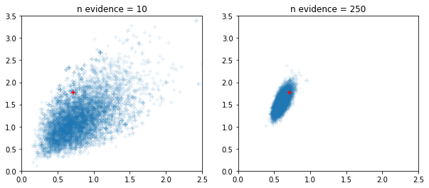
نمونهبردارهای HMC و NUTS تطبیقی پنجرهدار
fig, ax = plt.subplots(1, 2, figsize=(10, 4))
for i, n_evidence in enumerate((10, 250)):
  ax[i].set_title(f'n evidence = {n_evidence}')
  ax[i].set_xlim(0, 2.5); ax[i].set_ylim(0, 3.5)
  @tfd.JointDistributionCoroutine
  def model():
    Root = tfd.JointDistributionCoroutine.Root
    c0 = yield Root(tfd.Gamma(2, 2, name='c0'))
    c1 = yield Root(tfd.Gamma(2, 2, name='c1'))
    counts = yield tfd.Sample(tfd.BetaBinomial(23, c1, c0), n_evidence, name='counts')
  s = model.sample(seed=[20, 30])
  print(s)
  jd = model.experimental_pin(counts=s.counts)
  states, trace = tf.function(tfp.experimental.mcmc.windowed_adaptive_hmc)(
      100, jd, num_leapfrog_steps=5, seed=[100, 200])
  ax[i].scatter(states.c0.numpy().reshape(-1), states.c1.numpy().reshape(-1),
                marker='+', alpha=.1)
  ax[i].scatter(s.c0, s.c1, marker='+', color='r')
StructTuple(
  c0=<tf.Tensor: shape=(), dtype=float32, numpy=0.7161876>,
  c1=<tf.Tensor: shape=(), dtype=float32, numpy=1.7696666>,
  counts=<tf.Tensor: shape=(10,), dtype=float32, numpy=array([ 6., 10., 23.,  7.,  2., 20., 14., 16., 22., 17.], dtype=float32)>
)
WARNING:tensorflow:6 out of the last 6 calls to <function windowed_adaptive_hmc at 0x7fda42bed8c0> triggered tf.function retracing. Tracing is expensive and the excessive number of tracings could be due to (1) creating @tf.function repeatedly in a loop, (2) passing tensors with different shapes, (3) passing Python objects instead of tensors. For (1), please define your @tf.function outside of the loop. For (2), @tf.function has experimental_relax_shapes=True option that relaxes argument shapes that can avoid unnecessary retracing. For (3), please refer to https://www.tensorflow.org/guide/function#controlling_retracing and https://www.tensorflow.org/api_docs/python/tf/function for  more details.
StructTuple(
  c0=<tf.Tensor: shape=(), dtype=float32, numpy=0.7161876>,
  c1=<tf.Tensor: shape=(), dtype=float32, numpy=1.7696666>,
  counts=<tf.Tensor: shape=(250,), dtype=float32, numpy=
    array([ 6., 10., 23.,  7.,  2., 20., 14., 16., 22., 17., 22., 21.,  6.,
           21., 12., 22., 23., 16., 18., 21., 16., 17., 17., 16., 21., 14.,
           23., 15., 10., 19.,  8., 23., 23., 14.,  1., 23., 16., 22., 20.,
           20., 22., 15., 16., 20., 20., 21., 23., 22., 21., 15., 18., 23.,
           12., 16., 19., 23., 18.,  5., 22., 22., 22., 18., 12., 17., 17.,
           16.,  8., 22., 20., 23.,  3., 12., 14., 18.,  7., 19., 19.,  9.,
           10., 23., 14., 22., 22., 21., 13., 23., 14., 23., 10., 17., 23.,
           17., 20., 16., 20., 19., 14.,  0., 17., 22., 12.,  2., 17., 15.,
           14., 23., 19., 15., 23.,  2., 21., 23., 21.,  7., 21., 12., 23.,
           17., 17.,  4., 22., 16., 14., 19., 19., 20.,  6., 16., 14., 18.,
           21., 12., 21., 21., 22.,  2., 19., 11.,  6., 19.,  1., 23., 23.,
           14.,  6., 23., 18.,  8., 20., 23., 13., 20., 18., 23., 17., 22.,
           23., 20., 18., 22., 16., 23.,  9., 22., 21., 16., 20., 21., 16.,
           23.,  7., 13., 23., 19.,  3., 13., 23., 23., 13., 19., 23., 20.,
           18.,  8., 19., 14., 12.,  6.,  8., 23.,  3., 13., 21., 23., 22.,
           23., 19., 22., 21., 15., 22., 21., 21., 23.,  9., 19., 20., 23.,
           11., 23., 14., 23., 14., 21., 21., 10., 23.,  9., 13.,  1.,  8.,
            8., 20., 21., 21., 21., 14., 16., 16.,  9., 23., 22., 11., 23.,
           12., 18.,  1., 23.,  9.,  3., 21., 21., 23., 22., 18., 23., 16.,
            3., 11., 16.], dtype=float32)>
)
ریاضی، آمار
ریاضی/لینالگ
- اضافه کردن
tfp.math.trapzبرای یکپارچه سازی ذوزنقه. - اضافه کردن
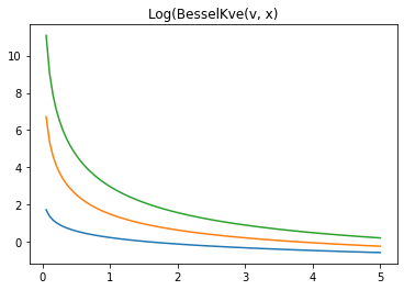
tfp.math.log_bessel_kve. - اضافه کردن
no_pivot_ldlبهexperimental.linalg. - اضافه کردن
marginal_fnآرگومان بهGaussianProcess(نگاه کنید بهno_pivot_ldl). - اضافه شده
tfp.math.atan_difference(x, y) - اضافه کردن
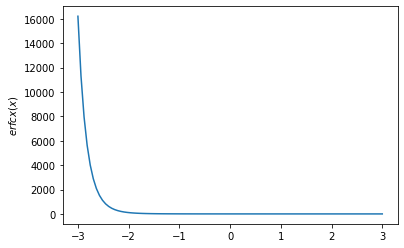
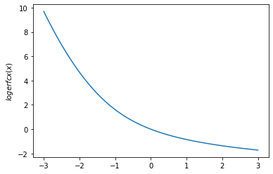
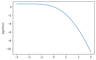
tfp.math.erfcx،tfp.math.logerfcوtfp.math.logerfcx - اضافه کردن
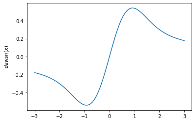
tfp.math.dawsnبرای انتگرال داوسون. - اضافه کردن
tfp.math.igammaincinv،tfp.math.igammacinv. - اضافه کردن
tfp.math.sqrt1pm1. - اضافه کردن
LogitNormal.stddev_approxوLogitNormal.variance_approx - اضافه کردن
tfp.math.owens_tبرای عملکرد آن T اوون است. - اضافه کردن
bracket_rootروش به مرزهای طور خودکار مقداردهی اولیه برای جستجوی ریشه. - روش Chandrupatla را برای یافتن ریشه توابع اسکالر اضافه کنید.
- اضافه کردن
آمار
-
tfp.stats.windowed_meanابزار موثر محاسبه پنجره. -
tfp.stats.windowed_varianceموثر و با دقت محاسبه پنجره واریانس. -
tfp.stats.cumulative_varianceموثر و با دقت محاسبه واریانس تجمعی. -
RunningCovarianceو دوستان هم اکنون می توانید از یک مثال تانسور مقدار دهی شود، نه تنها از شکل صریح و dtype. - تمیز کننده API برای
RunningCentralMoments،RunningMean،RunningPotentialScaleReduction.
-
توابع Owen's T، Erfcx، Logerfc، Logerfcx، Dawson
# Owen's T gives the probability that X > h, 0 < Y < a * X. Let's check that
# with random sampling.
h = np.array([1., 2.]).astype(np.float32)
a = np.array([10., 11.5]).astype(np.float32)
probs = tfp.math.owens_t(h, a)

x = tfd.Normal(0., 1.).sample(int(1e5), seed=(6, 245)).numpy()
y = tfd.Normal(0., 1.).sample(int(1e5), seed=(7, 245)).numpy()

true_values = (
    (x[..., np.newaxis] > h) &
    (0. < y[..., np.newaxis]) &
    (y[..., np.newaxis] < a * x[..., np.newaxis]))

print('Calculated values: {}'.format(
    np.count_nonzero(true_values, axis=0) / 1e5))

print('Expected values: {}'.format(probs))
Calculated values: [0.07896 0.01134]
Expected values: [0.07932763 0.01137507]
x = np.linspace(-3., 3., 100)
plt.plot(x, tfp.math.erfcx(x))
plt.ylabel('$erfcx(x)$')
plt.show()

plt.plot(x, tfp.math.logerfcx(x))
plt.ylabel('$logerfcx(x)$')
plt.show()

plt.plot(x, tfp.math.logerfc(x))
plt.ylabel('$logerfc(x)$')
plt.show()

plt.plot(x, tfp.math.dawsn(x))
plt.ylabel('$dawsn(x)$')
plt.show()
igammainv / igammacinv
# Igammainv and Igammacinv are inverses to Igamma and Igammac

x = np.linspace(1., 10., 10)
y = tf.math.igamma(0.3, x)
x_prime = tfp.math.igammainv(0.3, y)
print('x: {}'.format(x))
print('igammainv(igamma(a, x)):\n {}'.format(x_prime))

y = tf.math.igammac(0.3, x)
x_prime = tfp.math.igammacinv(0.3, y)

print('\n')
print('x: {}'.format(x))
print('igammacinv(igammac(a, x)):\n {}'.format(x_prime))
x: [ 1.  2.  3.  4.  5.  6.  7.  8.  9. 10.]
igammainv(igamma(a, x)):
 [1.        1.9999992 3.000003  4.0000024 5.0000257 5.999887  7.0002484
 7.999243  8.99872   9.994673 ]


x: [ 1.  2.  3.  4.  5.  6.  7.  8.  9. 10.]
igammacinv(igammac(a, x)):
 [1.       2.       3.       4.       5.       6.       7.       8.000001

 9.       9.999999]
log-kve
x = np.linspace(0., 5., 100)
for v in [0.5, 2., 3]:
  plt.plot(x, tfp.math.log_bessel_kve(v, x).numpy())

plt.title('Log(BesselKve(v, x)')
Text(0.5, 1.0, 'Log(BesselKve(v, x)')
دیگر
STS
- سرعت بخشیدن به پیش بینی و تجزیه STS با استفاده از داخلی
tf.functionبندی. - اضافه کردن گزینه برای سرعت بخشیدن به فیلترینگ در
LinearGaussianSSMهنگامی که نتایج تنها گام نهایی مورد نیاز است. - تغییرات استنتاج با توزیع های مشترک: به عنوان مثال نوت بوک با استفاده از مدل رادون .
- برای تبدیل هر توزیع به یک بیژکتور پیش شرطی، پشتیبانی آزمایشی را اضافه کنید.
- سرعت بخشیدن به پیش بینی و تجزیه STS با استفاده از داخلی
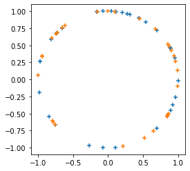
می افزاید
tfp.random.sanitize_seed.می افزاید
tfp.random.spherical_uniform.
plt.figure(figsize=(4, 4))
seed = tfp.random.sanitize_seed(123)
seed1, seed2 = tfp.random.split_seed(seed)
samps = tfp.random.spherical_uniform([30], dimension=2, seed=seed1)
plt.scatter(*samps.numpy().T, marker='+')
samps = tfp.random.spherical_uniform([30], dimension=2, seed=seed2)
plt.scatter(*samps.numpy().T, marker='+');