عفونت غیرمجاز و قابل توجه ، انتشار سریع کروناویروس جدید (SARS-CoV2) را تسهیل می کند

مشاهده در TensorFlow.org

در Google Colab اجرا شود

مشاهده منبع در GitHub

دانلود دفترچه یادداشت

این یک پورت احتمال TensorFlow از مقاله همنام 16 مارس 2020 توسط لی و همکاران است. ما صادقانه روش‌ها و نتایج نویسندگان اصلی را در پلتفرم TensorFlow Probability بازتولید می‌کنیم و برخی از قابلیت‌های TFP را در زمینه مدل‌سازی اپیدمیولوژی مدرن نشان می‌دهیم. انتقال به TensorFlow به ما سرعت 10 برابری نسبت به کد اصلی Matlab می دهد، و از آنجایی که TensorFlow Probability به طور فراگیر از محاسبات دسته ای برداری پشتیبانی می کند، همچنین به طور مطلوب به صدها تکرار مستقل مقیاس می شود.

کاغذ اصلی

روییون لی، سن پی، بن چن، ییمنگ سانگ، تائو ژانگ، وان یانگ و جفری شامان. عفونت غیرقانونی قابل توجهی انتشار سریع کروناویروس جدید (SARS-CoV2) را تسهیل می کند. (2020)، DOI: https://doi.org/10.1126/science.abb3221 .

چکیده: "برآورد میزان شیوع و سرایت از کروناویروس رمان (SARS-CoV2) عفونت مستند نشده برای درک شیوع کلی و پتانسیل همه گیر این بیماری بسیار مهم است در اینجا ما از مشاهدات از آلودگی گزارش شده در چین، در رابطه با داده تحرک، یک مدل فراجمعیت پویا شبکه‌ای و استنباط بیزی، برای استنتاج ویژگی‌های اپیدمیولوژیک مهم مرتبط با SARS-CoV2، از جمله بخش عفونت‌های غیرمستند و مسری بودن آن‌ها. ما تخمین می‌زنیم که 86 درصد از همه عفونت‌ها بدون سند بودند (95 درصد فاصله اطمینان (CI: [82-90 درصد]) ) قبل از محدودیت‌های سفر 23 ژانویه 2020. به ازای هر نفر، نرخ انتقال عفونت‌های غیرمستند 55 درصد از عفونت‌های ثبت‌شده ([46 تا 62 درصد]) بود، اما به دلیل تعداد بیشتر، عفونت‌های غیرمستند منبع عفونت برای 79 نفر بودند. درصد موارد ثبت شده. این یافته ها گسترش سریع جغرافیایی SARS-CoV2 را توضیح می دهد و نشان می دهد که مهار این ویروس به ویژه چالش برانگیز خواهد بود."

گیتهاب پیوند به کد و داده ها.

بررسی اجمالی

این مدل یک است مدل بیماری compartmental ، با محفظه برای "حساس"، "در معرض" (آلوده اما هنوز عفونی نیست)، "هرگز مستند های عفونی"، و "در نهایت مستند های عفونی". دو ویژگی قابل توجه وجود دارد: محفظه های جداگانه برای هر یک از 375 شهر چین، با فرضیاتی در مورد نحوه سفر مردم از شهری به شهر دیگر. و تاخیر در گزارش عفونت، به طوری که یک مورد است که می شود "در نهایت مستند های عفونی" در روز \(t\) می کند در تعداد مورد مشاهده شده را نشان نمی دهد تا یک روز بعد اتفاقی.

این مدل فرض می‌کند که مواردی که هرگز مستند نشده‌اند، به دلیل خفیف‌تر بودن، بدون سند پایان می‌یابند و در نتیجه دیگران را با سرعت کمتری آلوده می‌کنند. پارامتر اصلی مورد توجه در مقاله اصلی، نسبت مواردی است که مستند نشده است، تا هم میزان عفونت موجود و هم تأثیر انتقال غیرمستند بر گسترش بیماری را تخمین بزند.

این colab به عنوان یک مرور کد در سبک پایین به بالا ساختار یافته است. به ترتیب، ما

• داده ها را مصرف کنید و به طور خلاصه بررسی کنید،
• فضای حالت و دینامیک مدل را تعریف کنید،
• مجموعه ای از توابع را برای انجام استنتاج در مدلی که لی و همکارانش را دنبال می کند، بسازید
• آنها را فراخوانی کنید و نتایج را بررسی کنید. اسپویلر: همان کاغذ بیرون می آیند.

نصب و واردات پایتون

pip3 install -q tf-nightly tfp-nightly

import collections
import io
import requests
import time
import zipfile

import matplotlib.pyplot as plt
import numpy as np
import pandas as pd

import tensorflow.compat.v2 as tf
import tensorflow_probability as tfp
from tensorflow_probability.python.internal import samplers

tfd = tfp.distributions
tfes = tfp.experimental.sequential

واردات داده

بیایید داده ها را از github وارد کنیم و برخی از آنها را بررسی کنیم.

r = requests.get('https://raw.githubusercontent.com/SenPei-CU/COVID-19/master/Data.zip')
z = zipfile.ZipFile(io.BytesIO(r.content))
z.extractall('/tmp/')
raw_incidence = pd.read_csv('/tmp/data/Incidence.csv')
raw_mobility = pd.read_csv('/tmp/data/Mobility.csv')
raw_population = pd.read_csv('/tmp/data/pop.csv')

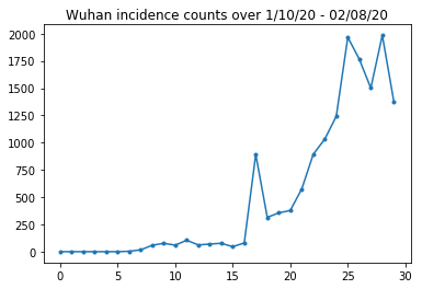
در زیر می توانیم تعداد بروز خام در روز را مشاهده کنیم. ما بیشتر به 14 روز اول (10 ژانویه تا 23 ژانویه) علاقه مند هستیم، زیرا محدودیت های سفر در 23 ژانویه اعمال شد. این مقاله با مدل‌سازی ژانویه 10-23 و ژانویه 23+ به طور جداگانه، با پارامترهای مختلف، به این موضوع می‌پردازد. ما فقط تولید مثل خود را به دوره قبلی محدود می کنیم.

raw_incidence.drop('Date', axis=1)  # The 'Date' column is all 1/18/21
# Luckily the days are in order, starting on January 10th, 2020.

بیایید میزان بروز ووهان را بررسی کنیم.

plt.plot(raw_incidence.Wuhan, '.-')
plt.title('Wuhan incidence counts over 1/10/20 - 02/08/20')
plt.show()

تا کنون خیلی خوب. اکنون جمعیت اولیه به حساب می آید.

raw_population

بیایید همچنین بررسی و ثبت کنیم که کدام ورودی ووهان است.

raw_population['City'][169]

'Wuhan'

WUHAN_IDX = 169

و در اینجا ماتریس تحرک بین شهرهای مختلف را می بینیم. این پروکسی برای تعداد افرادی است که در 14 روز اول بین شهرهای مختلف حرکت می کنند. این از سوابق GPS ارائه شده توسط Tencent برای فصل سال جدید قمری 2018 مشتق شده است. لی و همکاران تحرک مدل در طول فصل 2020 به عنوان برخی از ناشناخته (به استنتاج) ضریب ثابت \(\theta\) بار این.

raw_mobility

در نهایت، بیایید همه اینها را در آرایه‌های numpy که می‌توانیم مصرف کنیم، از قبل پردازش کنیم.

# The given populations are only "initial" because of intercity mobility during
# the holiday season.
initial_population = raw_population['Population'].to_numpy().astype(np.float32)

داده‌های تحرک را به یک تانسور [L، L، T] شکل تبدیل کنید، که L تعداد مکان‌ها و T تعداد گام‌های زمانی است.

daily_mobility_matrices = []
for i in range(1, 15):
  day_mobility = raw_mobility[raw_mobility['Day'] == i]

  # Make a matrix of daily mobilities.
  z = pd.crosstab(
      day_mobility.Origin, 
      day_mobility.Destination, 
      values=day_mobility['Mobility Index'], aggfunc='sum', dropna=False)

  # Include every city, even if there are no rows for some in the raw data on
  # some day.  This uses the sort order of `raw_population`.
  z = z.reindex(index=raw_population['City'], columns=raw_population['City'], 
                fill_value=0)
  # Finally, fill any missing entries with 0. This means no mobility.
  z = z.fillna(0)
  daily_mobility_matrices.append(z.to_numpy())

mobility_matrix_over_time = np.stack(daily_mobility_matrices, axis=-1).astype(
    np.float32)

در نهایت عفونت های مشاهده شده را بردارید و جدول [L, T] بسازید.

# Remove the date parameter and take the first 14 days.
observed_daily_infectious_count = raw_incidence.to_numpy()[:14, 1:]
observed_daily_infectious_count = np.transpose(
    observed_daily_infectious_count).astype(np.float32)

و دوباره بررسی کنید که شکل‌ها را آنطور که می‌خواستیم دریافت کرده‌ایم. برای یادآوری، ما با 375 شهر و 14 روز کار می کنیم.

print('Mobility Matrix over time should have shape (375, 375, 14): {}'.format(
    mobility_matrix_over_time.shape))
print('Observed Infectious should have shape (375, 14): {}'.format(
    observed_daily_infectious_count.shape))
print('Initial population should have shape (375): {}'.format(
    initial_population.shape))

Mobility Matrix over time should have shape (375, 375, 14): (375, 375, 14)
Observed Infectious should have shape (375, 14): (375, 14)
Initial population should have shape (375): (375,)

تعریف حالت و پارامترها

بیایید شروع به تعریف مدل خود کنیم. مدل ما بازتولید یک نوع از است مدل سیر . در این حالت ما حالت های متغیر زمانی زیر را داریم:

• \(S\): تعداد افراد مستعد به این بیماری در هر شهرستان.
• \(E\): تعداد افراد در هر شهرستان در معرض این بیماری عفونی، اما نکرده است. از نظر بیولوژیکی، این مربوط به ابتلا به این بیماری است، به طوری که همه افراد در معرض در نهایت عفونی می شوند.
• \(I^u\): تعداد افراد در هر شهرستان که مسری ولی مستند نشده است. در مدل، این در واقع به معنای "هرگز مستند نخواهد شد".
• \(I^r\): تعداد افراد در هر شهرستان که عفونی و مستند به عنوان چنین می باشد. لی و همکاران مدل تاخیر گزارش، پس \(I^r\) در واقع مربوط به چیزی شبیه به "مورد به اندازه کافی شدید در برخی از نقطه در آینده مستند شده است."

همانطور که در زیر خواهیم دید، ما این حالت ها را با اجرای فیلتر کالمن تنظیم شده توسط Ensemble (EAKF) به جلو در زمان استنتاج خواهیم کرد. بردار حالت EAKF برای هر یک از این کمیت ها یک بردار نمایه شهر است.

این مدل دارای پارامترهای جهانی قابل استنباط و متغیر زمان است:

• \(\beta\): نرخ انتقال با توجه به افراد عفونی مستند شده است.
• \(\mu\): نرخ انتقال از بستگانش به علت افراد بدون مدرک عفونی. این را از طریق کالا عمل \(\mu \beta\).
• \(\theta\): عامل تحرک بین شهری. این یک ضریب بزرگتر از یک تصحیح برای گزارش کمتر داده های تحرک (و برای رشد جمعیت از 2018 تا 2020) است.
• \(Z\): دوره کمون متوسط (به عنوان مثال، زمان در "در معرض" دولت).
• \(\alpha\): این کسری از عفونت های شدید به اندازه کافی به است (در نهایت) مستند شده است.
• \(D\): متوسط طول مدت زمان عفونت (به عنوان مثال، زمان در هر دو حالت "مسری").

ما تخمین‌های نقطه‌ای را برای این پارامترها با یک حلقه فیلترینگ تکراری در اطراف EAKF برای حالت‌ها استنباط خواهیم کرد.

این مدل همچنین به ثابت های استنتاج نشده بستگی دارد:

• \(M\): ماتریس تحرک بین شهری. این با زمان متغیر است و فرض می شود. به یاد بیاورید که آن را توسط استنباط پارامتر کوچک \(\theta\) به حرکت جمعیت واقعی بین شهرستانها.
• \(N\): تعداد کل افراد در هر شهرستان. جمعیت اولیه گرفته شده به عنوان داده می شود، و زمان تغییر جمعیت از اعداد تحرک محاسبه \(\theta M\).

ابتدا، ما به خودمان چند ساختار داده برای نگهداری حالت ها و پارامترهایمان می دهیم.

SEIRComponents = collections.namedtuple(
  typename='SEIRComponents',
  field_names=[
    'susceptible',              # S
    'exposed',                  # E
    'documented_infectious',    # I^r
    'undocumented_infectious',  # I^u
    # This is the count of new cases in the "documented infectious" compartment.
    # We need this because we will introduce a reporting delay, between a person
    # entering I^r and showing up in the observable case count data.
    # This can't be computed from the cumulative `documented_infectious` count,
    # because some portion of that population will move to the 'recovered'
    # state, which we aren't tracking explicitly.
    'daily_new_documented_infectious'])

ModelParams = collections.namedtuple(
    typename='ModelParams',
    field_names=[
      'documented_infectious_tx_rate',             # Beta
      'undocumented_infectious_tx_relative_rate',  # Mu
      'intercity_underreporting_factor',           # Theta
      'average_latency_period',                    # Z
      'fraction_of_documented_infections',         # Alpha
      'average_infection_duration'                 # D
    ]
)

ما همچنین مرزهای لی و همکاران را برای مقادیر پارامترها کد می کنیم.

PARAMETER_LOWER_BOUNDS = ModelParams(
    documented_infectious_tx_rate=0.8,
    undocumented_infectious_tx_relative_rate=0.2,
    intercity_underreporting_factor=1.,
    average_latency_period=2.,
    fraction_of_documented_infections=0.02,
    average_infection_duration=2.
)

PARAMETER_UPPER_BOUNDS = ModelParams(
    documented_infectious_tx_rate=1.5,
    undocumented_infectious_tx_relative_rate=1.,
    intercity_underreporting_factor=1.75,
    average_latency_period=5.,
    fraction_of_documented_infections=1.,
    average_infection_duration=5.
)

SEIR Dynamics

در اینجا ما رابطه بین پارامترها و حالت را تعریف می کنیم.

معادلات دینامیک زمان از Li و همکاران (مواد تکمیلی، معادلات 1-5) به شرح زیر است:

\(\frac{dS_i}{dt} = -\beta \frac{S_i I_i^r}{N_i} - \mu \beta \frac{S_i I_i^u}{N_i} + \theta \sum_k \frac{M_{ij} S_j}{N_j - I_j^r} - + \theta \sum_k \frac{M_{ji} S_j}{N_i - I_i^r}\)

\(\frac{dE_i}{dt} = \beta \frac{S_i I_i^r}{N_i} + \mu \beta \frac{S_i I_i^u}{N_i} -\frac{E_i}{Z} + \theta \sum_k \frac{M_{ij} E_j}{N_j - I_j^r} - + \theta \sum_k \frac{M_{ji} E_j}{N_i - I_i^r}\)

\(\frac{dI^r_i}{dt} = \alpha \frac{E_i}{Z} - \frac{I_i^r}{D}\)

\(\frac{dI^u_i}{dt} = (1 - \alpha) \frac{E_i}{Z} - \frac{I_i^u}{D} + \theta \sum_k \frac{M_{ij} I_j^u}{N_j - I_j^r} - + \theta \sum_k \frac{M_{ji} I^u_j}{N_i - I_i^r}\)

\(N_i = N_i + \theta \sum_j M_{ij} - \theta \sum_j M_{ji}\)

به عنوان یک یادآوری، \(i\) و \(j\) شهرستانها شاخص نویس. این معادلات تکامل زمانی بیماری را از طریق مدل سازی می کنند

• تماس با افراد عفونی که منجر به عفونت بیشتر می شود.
• پیشرفت بیماری از "در معرض" به یکی از حالت های "عفونی"؛
• پیشرفت بیماری از حالت‌های "عفونی" به بهبودی، که ما آن را با حذف از جمعیت مدل‌سازی شده مدل می‌کنیم.
• تحرک بین شهری، از جمله افراد آلوده یا غیرمجاز؛ و
• تغییرات زمانی جمعیت روزانه شهر از طریق تحرک بین شهری.

با پیروی از لی و همکاران، ما فرض می کنیم که افرادی که موارد آنقدر شدید است که در نهایت گزارش شود، بین شهرها سفر نمی کنند.

همچنین با پیروی از لی و همکاران، ما این دینامیک ها را تابع نویز پواسون از نظر اصطلاحی در نظر می گیریم، به عنوان مثال، هر عبارت در واقع نرخ پواسون است، نمونه ای از آن تغییر واقعی را نشان می دهد. نویز پواسون از نظر اصطلاحی است زیرا تفریق (در مقابل جمع کردن) نمونه‌های پواسون نتیجه توزیع شده توسط پواسون را به همراه نمی‌آورد.

ما این دینامیک ها را در زمان با انتگرالگر کلاسیک مرتبه چهارم Runge-Kutta تکامل خواهیم داد، اما ابتدا اجازه دهید تابعی را که آنها را محاسبه می کند (از جمله نمونه برداری از نویز پواسون) تعریف کنیم.

def sample_state_deltas(
    state, population, mobility_matrix, params, seed, is_deterministic=False):
  """Computes one-step change in state, including Poisson sampling.

  Note that this is coded to support vectorized evaluation on arbitrary-shape
  batches of states.  This is useful, for example, for running multiple
  independent replicas of this model to compute credible intervals for the
  parameters.  We refer to the arbitrary batch shape with the conventional
  `B` in the parameter documentation below.  This function also, of course,
  supports broadcasting over the batch shape.

  Args:
    state: A `SEIRComponents` tuple with fields Tensors of shape
      B + [num_locations] giving the current disease state.
    population: A Tensor of shape B + [num_locations] giving the current city
      populations.
    mobility_matrix: A Tensor of shape B + [num_locations, num_locations] giving
      the current baseline inter-city mobility.
    params: A `ModelParams` tuple with fields Tensors of shape B giving the
      global parameters for the current EAKF run.
    seed: Initial entropy for pseudo-random number generation.  The Poisson
      sampling is repeatable by supplying the same seed.
    is_deterministic: A `bool` flag to turn off Poisson sampling if desired.

  Returns:
    delta: A `SEIRComponents` tuple with fields Tensors of shape
      B + [num_locations] giving the one-day changes in the state, according
      to equations 1-4 above (including Poisson noise per Li et al).
  """
  undocumented_infectious_fraction = state.undocumented_infectious / population
  documented_infectious_fraction = state.documented_infectious / population

  # Anyone not documented as infectious is considered mobile
  mobile_population = (population - state.documented_infectious)
  def compute_outflow(compartment_population):
    raw_mobility = tf.linalg.matvec(
        mobility_matrix, compartment_population / mobile_population)
    return params.intercity_underreporting_factor * raw_mobility
  def compute_inflow(compartment_population):
    raw_mobility = tf.linalg.matmul(
        mobility_matrix,
        (compartment_population / mobile_population)[..., tf.newaxis],
        transpose_a=True)
    return params.intercity_underreporting_factor * tf.squeeze(
        raw_mobility, axis=-1)

  # Helper for sampling the Poisson-variate terms.
  seeds = samplers.split_seed(seed, n=11)
  if is_deterministic:
    def sample_poisson(rate):
      return rate
  else:
    def sample_poisson(rate):
      return tfd.Poisson(rate=rate).sample(seed=seeds.pop())

  # Below are the various terms called U1-U12 in the paper. We combined the
  # first two, which should be fine; both are poisson so their sum is too, and
  # there's no risk (as there could be in other terms) of going negative.
  susceptible_becoming_exposed = sample_poisson(
      state.susceptible *
      (params.documented_infectious_tx_rate *
       documented_infectious_fraction +
       (params.undocumented_infectious_tx_relative_rate *
        params.documented_infectious_tx_rate) *
       undocumented_infectious_fraction))  # U1 + U2

  susceptible_population_inflow = sample_poisson(
      compute_inflow(state.susceptible))  # U3
  susceptible_population_outflow = sample_poisson(
      compute_outflow(state.susceptible))  # U4

  exposed_becoming_documented_infectious = sample_poisson(
      params.fraction_of_documented_infections *
      state.exposed / params.average_latency_period)  # U5
  exposed_becoming_undocumented_infectious = sample_poisson(
      (1 - params.fraction_of_documented_infections) *
      state.exposed / params.average_latency_period)  # U6

  exposed_population_inflow = sample_poisson(
      compute_inflow(state.exposed))  # U7
  exposed_population_outflow = sample_poisson(
      compute_outflow(state.exposed))  # U8

  documented_infectious_becoming_recovered = sample_poisson(
      state.documented_infectious /
      params.average_infection_duration)  # U9
  undocumented_infectious_becoming_recovered = sample_poisson(
      state.undocumented_infectious /
      params.average_infection_duration)  # U10

  undocumented_infectious_population_inflow = sample_poisson(
      compute_inflow(state.undocumented_infectious))  # U11
  undocumented_infectious_population_outflow = sample_poisson(
      compute_outflow(state.undocumented_infectious))  # U12

  # The final state_deltas
  return SEIRComponents(
      # Equation [1]
      susceptible=(-susceptible_becoming_exposed +
                   susceptible_population_inflow +
                   -susceptible_population_outflow),
      # Equation [2]
      exposed=(susceptible_becoming_exposed +
               -exposed_becoming_documented_infectious +
               -exposed_becoming_undocumented_infectious +
               exposed_population_inflow +
               -exposed_population_outflow),
      # Equation [3]
      documented_infectious=(
          exposed_becoming_documented_infectious +
          -documented_infectious_becoming_recovered),
      # Equation [4]
      undocumented_infectious=(
          exposed_becoming_undocumented_infectious +
          -undocumented_infectious_becoming_recovered +
          undocumented_infectious_population_inflow +
          -undocumented_infectious_population_outflow),
      # New to-be-documented infectious cases, subject to the delayed
      # observation model.
      daily_new_documented_infectious=exposed_becoming_documented_infectious)

اینجا انتگرال است. این کاملا استاندارد، به جز برای عبور دانه PRNG از طریق به sample_state_deltas تابع به سر و صدا مستقل پواسون در هر یک از مراحل جزئی که رانگ روش Kutta تماس برای.

@tf.function(autograph=False)
def rk4_one_step(state, population, mobility_matrix, params, seed):
  """Implement one step of RK4, wrapped around a call to sample_state_deltas."""
  # One seed for each RK sub-step
  seeds = samplers.split_seed(seed, n=4)

  deltas = tf.nest.map_structure(tf.zeros_like, state)
  combined_deltas = tf.nest.map_structure(tf.zeros_like, state)

  for a, b in zip([1., 2, 2, 1.], [6., 3., 3., 6.]):
    next_input = tf.nest.map_structure(
        lambda x, delta, a=a: x + delta / a, state, deltas)
    deltas = sample_state_deltas(
        next_input,
        population,
        mobility_matrix,
        params,
        seed=seeds.pop(), is_deterministic=False)
    combined_deltas = tf.nest.map_structure(
        lambda x, delta, b=b: x + delta / b, combined_deltas, deltas)

  return tf.nest.map_structure(
      lambda s, delta: s + tf.round(delta),
      state, combined_deltas)

مقداردهی اولیه

در اینجا ما طرح اولیه سازی را از کاغذ پیاده سازی می کنیم.

به دنبال لی و همکاران، طرح استنتاج ما یک حلقه داخلی فیلتر کالمن تنظیم مجموعه خواهد بود که توسط یک حلقه فیلتر بیرونی تکرار شونده (IF-EAKF) احاطه شده است. از نظر محاسباتی، به این معنی است که ما به سه نوع مقداردهی اولیه نیاز داریم:

• حالت اولیه برای EAKF داخلی
• پارامترهای اولیه برای IF بیرونی، که پارامترهای اولیه برای اولین EAKF نیز هستند
• به روز رسانی پارامترها از یک تکرار IF به بعدی، که به عنوان پارامترهای اولیه برای هر EAKF غیر از اولی عمل می کند.

def initialize_state(num_particles, num_batches, seed):
  """Initialize the state for a batch of EAKF runs.

  Args:
    num_particles: `int` giving the number of particles for the EAKF.
    num_batches: `int` giving the number of independent EAKF runs to
      initialize in a vectorized batch.
    seed: PRNG entropy.

  Returns:
    state: A `SEIRComponents` tuple with Tensors of shape [num_particles,
      num_batches, num_cities] giving the initial conditions in each
      city, in each filter particle, in each batch member.
  """
  num_cities = mobility_matrix_over_time.shape[-2]
  state_shape = [num_particles, num_batches, num_cities]
  susceptible = initial_population * np.ones(state_shape, dtype=np.float32)
  documented_infectious = np.zeros(state_shape, dtype=np.float32)
  daily_new_documented_infectious = np.zeros(state_shape, dtype=np.float32)

  # Following Li et al, initialize Wuhan with up to 2000 people exposed
  # and another up to 2000 undocumented infectious.
  rng = np.random.RandomState(seed[0] % (2**31 - 1))
  wuhan_exposed = rng.randint(
      0, 2001, [num_particles, num_batches]).astype(np.float32)
  wuhan_undocumented_infectious = rng.randint(
      0, 2001, [num_particles, num_batches]).astype(np.float32)

  # Also following Li et al, initialize cities adjacent to Wuhan with three
  # days' worth of additional exposed and undocumented-infectious cases,
  # as they may have traveled there before the beginning of the modeling
  # period.
  exposed = 3 * mobility_matrix_over_time[
      WUHAN_IDX, :, 0] * wuhan_exposed[
          ..., np.newaxis] / initial_population[WUHAN_IDX]
  undocumented_infectious = 3 * mobility_matrix_over_time[
      WUHAN_IDX, :, 0] * wuhan_undocumented_infectious[
          ..., np.newaxis] / initial_population[WUHAN_IDX]

  exposed[..., WUHAN_IDX] = wuhan_exposed
  undocumented_infectious[..., WUHAN_IDX] = wuhan_undocumented_infectious

  # Following Li et al, we do not remove the inital exposed and infectious
  # persons from the susceptible population.
  return SEIRComponents(
      susceptible=tf.constant(susceptible),
      exposed=tf.constant(exposed),
      documented_infectious=tf.constant(documented_infectious),
      undocumented_infectious=tf.constant(undocumented_infectious),
      daily_new_documented_infectious=tf.constant(daily_new_documented_infectious))

def initialize_params(num_particles, num_batches, seed):
  """Initialize the global parameters for the entire inference run.

  Args:
    num_particles: `int` giving the number of particles for the EAKF.
    num_batches: `int` giving the number of independent EAKF runs to
      initialize in a vectorized batch.
    seed: PRNG entropy.

  Returns:
    params: A `ModelParams` tuple with fields Tensors of shape
      [num_particles, num_batches] giving the global parameters
      to use for the first batch of EAKF runs.
  """
  # We have 6 parameters. We'll initialize with a Sobol sequence,
  # covering the hyper-rectangle defined by our parameter limits.
  halton_sequence = tfp.mcmc.sample_halton_sequence(
      dim=6, num_results=num_particles * num_batches, seed=seed)
  halton_sequence = tf.reshape(
      halton_sequence, [num_particles, num_batches, 6])
  halton_sequences = tf.nest.pack_sequence_as(
      PARAMETER_LOWER_BOUNDS, tf.split(
          halton_sequence, num_or_size_splits=6, axis=-1))
  def interpolate(minval, maxval, h):
    return (maxval - minval) * h + minval
  return tf.nest.map_structure(
      interpolate,
      PARAMETER_LOWER_BOUNDS, PARAMETER_UPPER_BOUNDS, halton_sequences)

def update_params(num_particles, num_batches,
                  prev_params, parameter_variance, seed):
  """Update the global parameters between EAKF runs.

  Args:
    num_particles: `int` giving the number of particles for the EAKF.
    num_batches: `int` giving the number of independent EAKF runs to
      initialize in a vectorized batch.
    prev_params: A `ModelParams` tuple of the parameters used for the previous
      EAKF run.
    parameter_variance: A `ModelParams` tuple specifying how much to drift
      each parameter.
    seed: PRNG entropy.

  Returns:
    params: A `ModelParams` tuple with fields Tensors of shape
      [num_particles, num_batches] giving the global parameters
      to use for the next batch of EAKF runs.
  """
  # Initialize near the previous set of parameters. This is the first step
  # in Iterated Filtering.
  seeds = tf.nest.pack_sequence_as(
      prev_params, samplers.split_seed(seed, n=len(prev_params)))
  return tf.nest.map_structure(
      lambda x, v, seed: x + tf.math.sqrt(v) * tf.random.stateless_normal([
          num_particles, num_batches, 1], seed=seed),
      prev_params, parameter_variance, seeds)

تاخیر

یکی از ویژگی های مهم این مدل در نظر گرفتن صریح این واقعیت است که عفونت ها دیرتر از شروع گزارش می شوند. این است که، ما انتظار داریم که کسی که از حرکت می کند \(E\) محفظه به \(I^r\) محفظه در روز \(t\) ممکن است نشان نمی دهد تا در مشاهده تعداد مورد گزارش شده تا برخی از روز بعد.

ما تأخیر را توزیع گاما فرض می کنیم. با پیروی از لی و همکاران، ما از 1.85 برای شکل استفاده می کنیم و نرخ را پارامتر می کنیم تا متوسط ​​تاخیر گزارش دهی 9 روز را تولید کنیم.

def raw_reporting_delay_distribution(gamma_shape=1.85, reporting_delay=9.):
  return tfp.distributions.Gamma(
      concentration=gamma_shape, rate=gamma_shape / reporting_delay)

مشاهدات ما گسسته هستند، بنابراین تاخیرهای خام (پیوسته) را تا نزدیکترین روز گرد می کنیم. ما همچنین یک افق داده محدود داریم، بنابراین توزیع تاخیر برای یک فرد منفرد در روزهای باقی مانده یک طبقه بندی است. بنابراین ما می توانید در هر شهرستان مشاهدات پیش بینی بازده بیشتری نسبت به نمونه برداری محاسبه \(O(I^r)\) گاما، توسط احتمالات تاخیر چند جملهای های از پیش محاسبه به جای.

def reporting_delay_probs(num_timesteps, gamma_shape=1.85, reporting_delay=9.):
  gamma_dist = raw_reporting_delay_distribution(gamma_shape, reporting_delay)
  multinomial_probs = [gamma_dist.cdf(1.)]
  for k in range(2, num_timesteps + 1):
    multinomial_probs.append(gamma_dist.cdf(k) - gamma_dist.cdf(k - 1))
  # For samples that are larger than T.
  multinomial_probs.append(gamma_dist.survival_function(num_timesteps))
  multinomial_probs = tf.stack(multinomial_probs)
  return multinomial_probs

در اینجا کد اعمال این تأخیرها در شمارش‌های عفونی مستند روزانه جدید آمده است:

def delay_reporting(
    daily_new_documented_infectious, num_timesteps, t, multinomial_probs, seed):
  # This is the distribution of observed infectious counts from the current
  # timestep.

  raw_delays = tfd.Multinomial(
      total_count=daily_new_documented_infectious,
      probs=multinomial_probs).sample(seed=seed)

  # The last bucket is used for samples that are out of range of T + 1. Thus
  # they are not going to be observable in this model.
  clipped_delays = raw_delays[..., :-1]

  # We can also remove counts that are such that t + i >= T.
  clipped_delays = clipped_delays[..., :num_timesteps - t]
  # We finally shift everything by t. That means prepending with zeros.
  return tf.concat([
      tf.zeros(
          tf.concat([
              tf.shape(clipped_delays)[:-1], [t]], axis=0),
          dtype=clipped_delays.dtype),
      clipped_delays], axis=-1)

استنتاج

ابتدا چند ساختار داده را برای استنتاج تعریف می کنیم.

به طور خاص، ما می خواهیم فیلترینگ تکراری را انجام دهیم، که وضعیت و پارامترها را در حین انجام استنتاج با هم بسته بندی می کند. بنابراین ما یک تعریف ParameterStatePair شی.

ما همچنین می خواهیم هر گونه اطلاعات جانبی را به مدل بسته بندی کنیم.

ParameterStatePair = collections.namedtuple(
    'ParameterStatePair', ['state', 'params'])

# Info that is tracked and mutated but should not have inference performed over.
SideInfo = collections.namedtuple(
    'SideInfo', [
        # Observations at every time step.
        'observations_over_time',
        'initial_population',
        'mobility_matrix_over_time',
        'population',
        # Used for variance of measured observations.
        'actual_reported_cases',
        # Pre-computed buckets for the multinomial distribution.
        'multinomial_probs',
        'seed',
    ])

# Cities can not fall below this fraction of people
MINIMUM_CITY_FRACTION = 0.6

# How much to inflate the covariance by.
INFLATION_FACTOR = 1.1

INFLATE_FN = tfes.inflate_by_scaled_identity_fn(INFLATION_FACTOR)

در اینجا مدل مشاهده کامل، بسته بندی شده برای فیلتر Ensemble Kalman است.

ویژگی جالب تأخیرهای گزارش دهی (محاسبه شده مانند قبل) است. مدل بالادست ساطع می کند daily_new_documented_infectious برای هر شهرستان در هر مرحله زمان.

# We observe the observed infections.
def observation_fn(t, state_params, extra):
  """Generate reported cases.

  Args:
    state_params: A `ParameterStatePair` giving the current parameters
      and state.
    t: Integer giving the current time.
    extra: A `SideInfo` carrying auxiliary information.

  Returns:
    observations: A Tensor of predicted observables, namely new cases
      per city at time `t`.
    extra: Update `SideInfo`.
  """
  # Undo padding introduced in `inference`.
  daily_new_documented_infectious = state_params.state.daily_new_documented_infectious[..., 0]
  # Number of people that we have already committed to become
  # observed infectious over time.
  # shape: batch + [num_particles, num_cities, time]
  observations_over_time = extra.observations_over_time
  num_timesteps = observations_over_time.shape[-1]

  seed, new_seed = samplers.split_seed(extra.seed, salt='reporting delay')

  daily_delayed_counts = delay_reporting(
      daily_new_documented_infectious, num_timesteps, t,
      extra.multinomial_probs, seed)
  observations_over_time = observations_over_time + daily_delayed_counts

  extra = extra._replace(
      observations_over_time=observations_over_time,
      seed=new_seed)

  # Actual predicted new cases, re-padded.
  adjusted_observations = observations_over_time[..., t][..., tf.newaxis]
  # Finally observations have variance that is a function of the true observations:
  return tfd.MultivariateNormalDiag(
      loc=adjusted_observations,
      scale_diag=tf.math.maximum(
          2., extra.actual_reported_cases[..., t][..., tf.newaxis] / 2.)), extra

در اینجا ما دینامیک انتقال را تعریف می کنیم. ما قبلاً کار معنایی را انجام داده ایم. در اینجا ما فقط آن را برای چارچوب EAKF بسته بندی می کنیم، و با پیروی از لی و همکاران، جمعیت شهرها را برای جلوگیری از کوچک شدن بیش از حد آنها، کلیپ می کنیم.

def transition_fn(t, state_params, extra):
  """SEIR dynamics.

  Args:
    state_params: A `ParameterStatePair` giving the current parameters
      and state.
    t: Integer giving the current time.
    extra: A `SideInfo` carrying auxiliary information.

  Returns:
    state_params: A `ParameterStatePair` predicted for the next time step.
    extra: Updated `SideInfo`.
  """
  mobility_t = extra.mobility_matrix_over_time[..., t]
  new_seed, rk4_seed = samplers.split_seed(extra.seed, salt='Transition')
  new_state = rk4_one_step(
      state_params.state,
      extra.population,
      mobility_t,
      state_params.params,
      seed=rk4_seed)

  # Make sure population doesn't go below MINIMUM_CITY_FRACTION.
  new_population = (
      extra.population + state_params.params.intercity_underreporting_factor * (
          # Inflow
          tf.reduce_sum(mobility_t, axis=-2) - 
          # Outflow
          tf.reduce_sum(mobility_t, axis=-1)))
  new_population = tf.where(
      new_population < MINIMUM_CITY_FRACTION * extra.initial_population,
      extra.initial_population * MINIMUM_CITY_FRACTION,
      new_population)

  extra = extra._replace(population=new_population, seed=new_seed)

  # The Ensemble Kalman Filter code expects the transition function to return a distribution.
  # As the dynamics and noise are encapsulated above, we construct a `JointDistribution` that when
  # sampled, returns the values above.

  new_state = tfd.JointDistributionNamed(
      model=tf.nest.map_structure(lambda x: tfd.VectorDeterministic(x), new_state))
  params = tfd.JointDistributionNamed(
      model=tf.nest.map_structure(lambda x: tfd.VectorDeterministic(x), state_params.params))

  state_params = tfd.JointDistributionNamed(
      model=ParameterStatePair(state=new_state, params=params))

  return state_params, extra

در نهایت روش استنتاج را تعریف می کنیم. این دو حلقه است، حلقه بیرونی Iterated Filtering است در حالی که حلقه داخلی Ensemble Adjustment Kalman Filtering است.

# Use tf.function to speed up EAKF prediction and updates.
ensemble_kalman_filter_predict = tf.function(
    tfes.ensemble_kalman_filter_predict, autograph=False)
ensemble_adjustment_kalman_filter_update = tf.function(
    tfes.ensemble_adjustment_kalman_filter_update, autograph=False)

def inference(
    num_ensembles,
    num_batches,
    num_iterations,
    actual_reported_cases,
    mobility_matrix_over_time,
    seed=None,
    # This is how much to reduce the variance by in every iterative
    # filtering step.
    variance_shrinkage_factor=0.9,
    # Days before infection is reported.
    reporting_delay=9.,
    # Shape parameter of Gamma distribution.
    gamma_shape_parameter=1.85):
  """Inference for the Shaman, et al. model.

  Args:
    num_ensembles: Number of particles to use for EAKF.
    num_batches: Number of batches of IF-EAKF to run.
    num_iterations: Number of iterations to run iterative filtering.
    actual_reported_cases: `Tensor` of shape `[L, T]` where `L` is the number
      of cities, and `T` is the timesteps.
    mobility_matrix_over_time: `Tensor` of shape `[L, L, T]` which specifies the
      mobility between locations over time.
    variance_shrinkage_factor: Python `float`. How much to reduce the
      variance each iteration of iterated filtering.
    reporting_delay: Python `float`. How many days before the infection
      is reported.
    gamma_shape_parameter: Python `float`. Shape parameter of Gamma distribution
      of reporting delays.

  Returns:
    result: A `ModelParams` with fields Tensors of shape [num_batches],
      containing the inferred parameters at the final iteration.
  """
  print('Starting inference.')
  num_timesteps = actual_reported_cases.shape[-1]
  params_per_iter = []

  multinomial_probs = reporting_delay_probs(
      num_timesteps, gamma_shape_parameter, reporting_delay)

  seed = samplers.sanitize_seed(seed, salt='Inference')

  for i in range(num_iterations):
    start_if_time = time.time()
    seeds = samplers.split_seed(seed, n=4, salt='Initialize')
    if params_per_iter:
      parameter_variance = tf.nest.map_structure(
          lambda minval, maxval: variance_shrinkage_factor ** (
              2 * i) * (maxval - minval) ** 2 / 4.,
          PARAMETER_LOWER_BOUNDS, PARAMETER_UPPER_BOUNDS)
      params_t = update_params(
          num_ensembles,
          num_batches,
          prev_params=params_per_iter[-1],
          parameter_variance=parameter_variance,
          seed=seeds.pop())
    else:
      params_t = initialize_params(num_ensembles, num_batches, seed=seeds.pop())

    state_t = initialize_state(num_ensembles, num_batches, seed=seeds.pop())
    population_t = sum(x for x in state_t)
    observations_over_time = tf.zeros(
        [num_ensembles,
         num_batches,
         actual_reported_cases.shape[0], num_timesteps])

    extra = SideInfo(
        observations_over_time=observations_over_time,
        initial_population=tf.identity(population_t),
        mobility_matrix_over_time=mobility_matrix_over_time,
        population=population_t,
        multinomial_probs=multinomial_probs,
        actual_reported_cases=actual_reported_cases,
        seed=seeds.pop())

    # Clip states
    state_t = clip_state(state_t, population_t)
    params_t = clip_params(params_t, seed=seeds.pop())

    # Accrue the parameter over time. We'll be averaging that
    # and using that as our MLE estimate.
    params_over_time = tf.nest.map_structure(
        lambda x: tf.identity(x), params_t)

    state_params = ParameterStatePair(state=state_t, params=params_t)

    eakf_state = tfes.EnsembleKalmanFilterState(
        step=tf.constant(0), particles=state_params, extra=extra)

    for j in range(num_timesteps):
      seeds = samplers.split_seed(eakf_state.extra.seed, n=3)

      extra = extra._replace(seed=seeds.pop())

      # Predict step.

      # Inflate and clip.
      new_particles = INFLATE_FN(eakf_state.particles)
      state_t = clip_state(new_particles.state, eakf_state.extra.population)
      params_t = clip_params(new_particles.params, seed=seeds.pop())
      eakf_state = eakf_state._replace(
          particles=ParameterStatePair(params=params_t, state=state_t))

      eakf_predict_state = ensemble_kalman_filter_predict(eakf_state, transition_fn)

      # Clip the state and particles.
      state_params = eakf_predict_state.particles
      state_t = clip_state(
          state_params.state, eakf_predict_state.extra.population)
      state_params = ParameterStatePair(state=state_t, params=state_params.params)

      # We preprocess the state and parameters by affixing a 1 dimension. This is because for
      # inference, we treat each city as independent. We could also introduce localization by
      # considering cities that are adjacent.
      state_params = tf.nest.map_structure(lambda x: x[..., tf.newaxis], state_params)
      eakf_predict_state = eakf_predict_state._replace(particles=state_params)

      # Update step.

      eakf_update_state = ensemble_adjustment_kalman_filter_update(
          eakf_predict_state,
          actual_reported_cases[..., j][..., tf.newaxis],
          observation_fn)

      state_params = tf.nest.map_structure(
          lambda x: x[..., 0], eakf_update_state.particles)

      # Clip to ensure parameters / state are well constrained.
      state_t = clip_state(
          state_params.state, eakf_update_state.extra.population)

      # Finally for the parameters, we should reduce over all updates. We get
      # an extra dimension back so let's do that.
      params_t = tf.nest.map_structure(
          lambda x, y: x + tf.reduce_sum(y[..., tf.newaxis] - x, axis=-2, keepdims=True),
          eakf_predict_state.particles.params, state_params.params)
      params_t = clip_params(params_t, seed=seeds.pop())
      params_t = tf.nest.map_structure(lambda x: x[..., 0], params_t)

      state_params = ParameterStatePair(state=state_t, params=params_t)
      eakf_state = eakf_update_state
      eakf_state = eakf_state._replace(particles=state_params)

      # Flatten and collect the inferred parameter at time step t.
      params_over_time = tf.nest.map_structure(
          lambda s, x: tf.concat([s, x], axis=-1), params_over_time, params_t)

    est_params = tf.nest.map_structure(
        # Take the average over the Ensemble and over time.
        lambda x: tf.math.reduce_mean(x, axis=[0, -1])[..., tf.newaxis],
        params_over_time)
    params_per_iter.append(est_params)
    print('Iterated Filtering {} / {} Ran in: {:.2f} seconds'.format(
        i, num_iterations, time.time() - start_if_time))

  return tf.nest.map_structure(
      lambda x: tf.squeeze(x, axis=-1), params_per_iter[-1])

جزئیات نهایی: برش پارامترها و وضعیت شامل اطمینان از اینکه آنها در محدوده هستند و غیر منفی هستند.

def clip_state(state, population):
  """Clip state to sensible values."""
  state = tf.nest.map_structure(
      lambda x: tf.where(x < 0, 0., x), state)

  # If S > population, then adjust as well.
  susceptible = tf.where(state.susceptible > population, population, state.susceptible)
  return SEIRComponents(
      susceptible=susceptible,
      exposed=state.exposed,
      documented_infectious=state.documented_infectious,
      undocumented_infectious=state.undocumented_infectious,
      daily_new_documented_infectious=state.daily_new_documented_infectious)

def clip_params(params, seed):
  """Clip parameters to bounds."""
  def _clip(p, minval, maxval):
    return tf.where(
        p < minval,
        minval * (1. + 0.1 * tf.random.stateless_uniform(p.shape, seed=seed)),
        tf.where(p > maxval,
                 maxval * (1. - 0.1 * tf.random.stateless_uniform(
                     p.shape, seed=seed)), p))
  params = tf.nest.map_structure(
      _clip, params, PARAMETER_LOWER_BOUNDS, PARAMETER_UPPER_BOUNDS)

  return params

اجرای آن همه با هم

# Let's sample the parameters.
#
# NOTE: Li et al. run inference 1000 times, which would take a few hours.
# Here we run inference 30 times (in a single, vectorized batch).
best_parameters = inference(
    num_ensembles=300,
    num_batches=30,
    num_iterations=10,
    actual_reported_cases=observed_daily_infectious_count,
    mobility_matrix_over_time=mobility_matrix_over_time)

Starting inference.
Iterated Filtering 0 / 10 Ran in: 26.65 seconds
Iterated Filtering 1 / 10 Ran in: 28.69 seconds
Iterated Filtering 2 / 10 Ran in: 28.06 seconds
Iterated Filtering 3 / 10 Ran in: 28.48 seconds
Iterated Filtering 4 / 10 Ran in: 28.57 seconds
Iterated Filtering 5 / 10 Ran in: 28.35 seconds
Iterated Filtering 6 / 10 Ran in: 28.35 seconds
Iterated Filtering 7 / 10 Ran in: 28.19 seconds
Iterated Filtering 8 / 10 Ran in: 28.58 seconds
Iterated Filtering 9 / 10 Ran in: 28.23 seconds

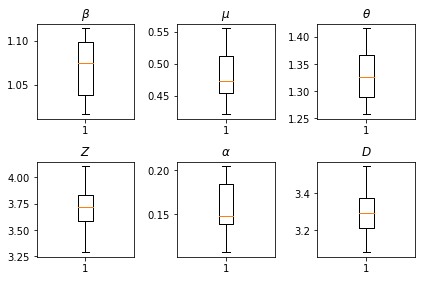
نتایج استنباطات ما ما در بر ارزش حداکثر احتمال رسم برای همه پارامترهای جهانی نشان می دهد تنوع خود را در سراسر ما num_batches اجرا می شود مستقل از استنتاج است. این با جدول S1 در مواد تکمیلی مطابقت دارد.

fig, axs = plt.subplots(2, 3)
axs[0, 0].boxplot(best_parameters.documented_infectious_tx_rate,
                  whis=(2.5,97.5), sym='')
axs[0, 0].set_title(r'$\beta$')

axs[0, 1].boxplot(best_parameters.undocumented_infectious_tx_relative_rate,
                  whis=(2.5,97.5), sym='')
axs[0, 1].set_title(r'$\mu$')

axs[0, 2].boxplot(best_parameters.intercity_underreporting_factor,
                  whis=(2.5,97.5), sym='')
axs[0, 2].set_title(r'$\theta$')

axs[1, 0].boxplot(best_parameters.average_latency_period,
                  whis=(2.5,97.5), sym='')
axs[1, 0].set_title(r'$Z$')

axs[1, 1].boxplot(best_parameters.fraction_of_documented_infections,
                  whis=(2.5,97.5), sym='')
axs[1, 1].set_title(r'$\alpha$')

axs[1, 2].boxplot(best_parameters.average_infection_duration,
                  whis=(2.5,97.5), sym='')
axs[1, 2].set_title(r'$D$')
plt.tight_layout()