การอนุมานแบบแปรผันบนแบบจำลองกราฟิกความน่าจะเป็นที่มีการแจกแจงร่วม

ดูบน TensorFlow.org

ทำงานใน Google Colab

ดูแหล่งที่มาบน GitHub

ดาวน์โหลดโน๊ตบุ๊ค

Variational Inference (VI) ใช้การอนุมานแบบเบย์โดยประมาณว่าเป็นปัญหาการปรับให้เหมาะสมที่สุด และพยายามหาการกระจายแบบหลัง 'ตัวแทน' ที่ลดความแตกต่างของ KL กับส่วนหลังที่แท้จริง VI แบบไล่ระดับมักจะเร็วกว่าวิธี MCMC ซึ่งประกอบขึ้นเองตามธรรมชาติด้วยการปรับพารามิเตอร์แบบจำลองให้เหมาะสมที่สุด และให้ขอบเขตที่ต่ำกว่าในหลักฐานแบบจำลองที่สามารถนำมาใช้โดยตรงสำหรับการเปรียบเทียบแบบจำลอง การวินิจฉัยการลู่เข้า และการอนุมานที่ประกอบได้

ความน่าจะเป็นของ TensorFlow นำเสนอเครื่องมือสำหรับ VI ที่รวดเร็ว ยืดหยุ่น และปรับขนาดได้ซึ่งพอดีกับสแต็ก TFP อย่างเป็นธรรมชาติ เครื่องมือเหล่านี้ช่วยให้สามารถสร้างส่วนหลังของตัวแทนเสมือนที่มีโครงสร้างความแปรปรวนร่วมที่เกิดจากการแปลงเชิงเส้นหรือกระแสการทำให้เป็นมาตรฐาน

VI สามารถนำมาใช้ในการประมาณการคชกรรม ช่วงเวลาที่น่าเชื่อถือ สำหรับพารามิเตอร์ของรูปแบบการถดถอยที่จะประเมินผลกระทบของการรักษาต่างๆหรือคุณลักษณะสังเกตเกี่ยวกับผลของดอกเบี้ย ช่วงที่น่าเชื่อถือผูกมัดค่าของพารามิเตอร์ที่ไม่ได้สังเกตด้วยความน่าจะเป็นที่แน่นอน ตามการแจกแจงหลังของพารามิเตอร์ที่ปรับเงื่อนไขกับข้อมูลที่สังเกตได้ และให้สมมติฐานเกี่ยวกับการแจกแจงก่อนหน้าของพารามิเตอร์

ใน Colab นี้เราแสดงให้เห็นถึงวิธีการใช้ VI ที่จะได้รับช่วงเวลาที่น่าเชื่อถือสำหรับพารามิเตอร์ของคชกรรมเชิงเส้นแบบการถดถอยในระดับเรดอนวัดในบ้าน (โดยใช้ Gelman et al, ของ (2007) ชุดเรดอน. ดู ตัวอย่างที่คล้ายกัน ในสแตน) เราแสดงให้เห็นว่า TFP JointDistribution s รวมกับ bijectors ในการสร้างและพอดีกับสองประเภทของ posteriors ตัวแทนแสดงออก:

• การแจกแจงแบบปกติมาตรฐานที่แปลงโดยบล็อกเมทริกซ์ เมทริกซ์อาจสะท้อนถึงความเป็นอิสระในองค์ประกอบบางอย่างของส่วนหลังและการพึ่งพาอาศัยกัน เป็นการผ่อนคลายสมมติฐานของค่าความแปรปรวนร่วมหรือค่าความแปรปรวนร่วมแบบเต็ม
• ที่มีความซับซ้อนมากขึ้นความจุสูงกว่า ผกผันไหลอัต

หลังของตัวแทนเสมือนได้รับการฝึกฝนและเปรียบเทียบกับผลลัพธ์จากการตรวจวัดพื้นฐานด้านหลังตัวแทนเสมือนในสนาม เช่นเดียวกับตัวอย่างจากความจริงภาคพื้นดินจากแฮมิลตันเนียน มอนติคาร์โล

ภาพรวมของการอนุมานแบบแปรผันแบบเบย์

สมมติว่าเรามีขั้นตอนการกำเนิดต่อไปนี้ที่ \(\theta\) หมายถึงพารามิเตอร์สุ่ม \(\omega\) หมายถึงค่าพารามิเตอร์ที่กำหนดและ \(x_i\) มีคุณสมบัติและ \(y_i\) เป็นค่าเป้าหมายสำหรับการ \(i=1,\ldots,n\) สังเกตจุดข้อมูล: \ begin {ชิด } &\theta \sim r(\Theta) && \text{(Prior)}\ &\text{for } i = 1 \ldots n: \nonumber \ &\quad y_i \sim p(Y_i|x_i, \theta \ โอเมก้า) && \ ข้อความ {(โอกาส)} \ end {} ชิด

VI มีลักษณะดังนี้: $\newcommand{\E}{\operatorname{\mathbb{E} } } \newcommand{\K}{\operatorname{\mathbb{K} } } \newcommand{\defeq}{\overset {\tiny\text{def} }{=} } \DeclareMathOperator*{\argmin}{arg\,min}$

\ begin {จัด} - \ บันทึก P ({y_i} _i ^ n | {x_i} _i ^ n, \ omega) และ \ defeq - \ Log \ int \ textrm {d} \ theta \ r (\ theta) \ prod_i^np(y_i|x_i,\theta, \omega) && \text{(อินทิกรัลที่ยากมาก)} \ &= -\log \int \textrm{d}\theta\, q(\theta) \frac{1 }{q(\theta)} r(\theta) \prod_i^np(y_i|x_i,\theta, \omega) && \text{(คูณด้วย 1)}\ &\le - \int \textrm{d} \ theta \, Q (\ theta) \ Log \ frac {r (\ theta) \ prod_i ^ NP (y_i | x i, \ theta, \ omega)} {Q (\ theta)} && \ ข้อความ {(ความไม่เท่าเทียมกันของเซ่น )} \ & \ defeq \ E {Q (\ ที)} [- \ บันทึก P (y_i | x_i \ ที \ omega)] + \ K [Q (\ ที) R (\ ที)] \ & \ defeq \text{expected negative log likelihood"} + ปลาย \ ข้อความ {regularizer kl"} \ {} ชิด

(ในทางเทคนิคเราสมมติ \(q\) เป็น อย่างต่อเนื่อง เกี่ยวกับการ \(r\). ดูยัง ความไม่เท่าเทียมกันของเซ่น .)

เนื่องจากขอบเขตถือสำหรับ q ทั้งหมด จึงชัดเจนที่สุดสำหรับ:

\[q^*,w^* = \argmin_{q \in \mathcal{Q},\omega\in\mathbb{R}^d} \left\{ \sum_i^n\E_{q(\Theta)}\left[ -\log p(y_i|x_i,\Theta, \omega) \right] + \K[q(\Theta), r(\Theta)] \right\}\]

เกี่ยวกับคำศัพท์เราเรียกว่า

• \(q^*\) ว่า "หลังตัวแทน" และ
• \(\mathcal{Q}\) ว่า "ครอบครัวตัวแทน."

\(\omega^*\) หมายถึงค่าโอกาสสูงสุดของพารามิเตอร์ที่กำหนดเกี่ยวกับการสูญเสียที่หก ดู การสำรวจครั้งนี้ สำหรับข้อมูลเพิ่มเติมเกี่ยวกับการอนุมานแปรผัน

ตัวอย่าง: การถดถอยเชิงเส้นแบบลำดับชั้นแบบเบย์ในการวัดเรดอน

เรดอนเป็นก๊าซกัมมันตภาพรังสีที่เข้าสู่บ้านเรือนผ่านจุดสัมผัสพื้น เป็นสารก่อมะเร็งที่เป็นสาเหตุหลักของมะเร็งปอดในผู้ไม่สูบบุหรี่ ระดับเรดอนแตกต่างกันไปในแต่ละครัวเรือน

EPA ได้ทำการศึกษาระดับเรดอนในบ้าน 80,000 หลัง ตัวทำนายที่สำคัญสองประการคือ:

• ชั้นที่ใช้วัด (เรดอนสูงกว่าในห้องใต้ดิน)
• ระดับยูเรเนียมในเขต (ความสัมพันธ์เชิงบวกกับระดับเรดอน)

ทำนายระดับเรดอนในบ้านจัดกลุ่มตามเขตที่เป็นปัญหาคลาสสิกในการสร้างแบบจำลองคชกรรมลำดับชั้นนำโดย Gelman และฮิลล์ (2006) เราจะสร้างแบบจำลองเชิงเส้นแบบลำดับชั้นเพื่อทำนายการวัดเรดอนในบ้าน ซึ่งลำดับชั้นคือการจัดกลุ่มบ้านตามเขต เรามีความสนใจในช่วงเวลาที่น่าเชื่อถือสำหรับผลกระทบของสถานที่ (เคาน์ตี) ต่อระดับเรดอนของบ้านในมินนิโซตา เพื่อแยกผลกระทบนี้ แบบจำลองจะรวมผลกระทบของระดับพื้นและยูเรเนียมไว้ด้วย นอกจากนี้ เราจะรวมผลกระทบตามบริบทที่สอดคล้องกับพื้นเฉลี่ยที่ใช้การวัดโดยเคาน์ตี เพื่อที่ว่าหากมีความแตกต่างระหว่างเคาน์ตีของพื้นที่ซึ่งใช้การวัด ค่านี้ไม่ได้เกิดจากผลกระทบของเคาน์ตี

pip3 install -q tf-nightly tfp-nightly

import matplotlib.pyplot as plt
import numpy as np
import seaborn as sns
import tensorflow as tf
import tensorflow_datasets as tfds
import tensorflow_probability as tfp
import warnings

tfd = tfp.distributions
tfb = tfp.bijectors

plt.rcParams['figure.facecolor'] = '1.'

# Load the Radon dataset from `tensorflow_datasets` and filter to data from
# Minnesota.
dataset = tfds.as_numpy(
    tfds.load('radon', split='train').filter(
        lambda x: x['features']['state'] == 'MN').batch(10**9))

# Dependent variable: Radon measurements by house.
dataset = next(iter(dataset))
radon_measurement = dataset['activity'].astype(np.float32)
radon_measurement[radon_measurement <= 0.] = 0.1
log_radon = np.log(radon_measurement)

# Measured uranium concentrations in surrounding soil.
uranium_measurement = dataset['features']['Uppm'].astype(np.float32)
log_uranium = np.log(uranium_measurement)

# County indicator.
county_strings = dataset['features']['county'].astype('U13')
unique_counties, county = np.unique(county_strings, return_inverse=True)
county = county.astype(np.int32)
num_counties = unique_counties.size

# Floor on which the measurement was taken.
floor_of_house = dataset['features']['floor'].astype(np.int32)

# Average floor by county (contextual effect).
county_mean_floor = []
for i in range(num_counties):
  county_mean_floor.append(floor_of_house[county == i].mean())
county_mean_floor = np.array(county_mean_floor, dtype=log_radon.dtype)
floor_by_county = county_mean_floor[county]

แบบจำลองการถดถอยมีการระบุดังนี้:

\(\newcommand{\Normal}{\operatorname{\sf Normal} }\)\ begin {จัด} & \ ข้อความ {uranium_weight} \ ซิม \ ปกติ (0, 1) \ & \ ข้อความ {county_floor_weight} \ ซิม \ ปกติ (0, 1) \ & \ ข้อความ {สำหรับ} J = 1 \ ldots \text{num_counties}:\ &\quad \text{county_effect}_j \sim \Normal (0, \sigma_c)\ &\text{for } i = 1\ldots n:\ &\quad \mu_i = ( \ และ \ สี่เหลี่ยม \ สี่เหลี่ยม \ ข้อความ {อคติ} \ และ \ สี่เหลี่ยม \ สี่เหลี่ยม + \ ข้อความ {ผลเขต} {\ ข้อความ {เขต} _i} \ และ \ สี่เหลี่ยม \ สี่เหลี่ยม + \ ข้อความ {log_uranium} _i \ ข้อความครั้ง \ {uranium_weight } \ และ \ สี่เหลี่ยม \ สี่เหลี่ยม + \ ข้อความ {floor_of_house} _i \ times \ ข้อความ {floor_weight} \ และ \ สี่เหลี่ยม \ สี่เหลี่ยม + \ ข้อความ {floor_by เขต} {\ ข้อความ {เขต} _i} \ ข้อความครั้ง \ {county_floor_weight}) \ & \ สี่เหลี่ยม \ ข้อความ {log_radon} _i \ ซิม \ ปกติ (\ mu_i \ sigma_y) \ end {จัด} ซึ่ง \(i\) ดัชนีสังเกตและ \(\text{county}_i\) เป็นเขตที่ \(i\)สังเกต TH เป็น ถ่าย.

เราใช้เอฟเฟกต์สุ่มระดับเคาน์ตีเพื่อบันทึกความผันแปรทางภูมิศาสตร์ พารามิเตอร์ uranium_weight และ county_floor_weight ย่อม probabilistically และ floor_weight และคง bias มีกำหนด ตัวเลือกการสร้างแบบจำลองเหล่านี้มักเกิดขึ้นโดยพลการ และจัดทำขึ้นเพื่อจุดประสงค์ในการสาธิต VI บนแบบจำลองความน่าจะเป็นของความซับซ้อนที่เหมาะสม สำหรับการอภิปรายอย่างละเอียดมากขึ้นของการสร้างแบบจำลองหลายระดับที่มีผลกระทบคงที่และแบบสุ่มใน TFP โดยใช้ชุดข้อมูลเรดอนดู หลายแบบจำลองรองพื้น และ ฟิตติ้งเชิงเส้นทั่วไปผสมผลรุ่นใช้แปรผันอนุมาน

# Create variables for fixed effects.
floor_weight = tf.Variable(0.)
bias = tf.Variable(0.)

# Variables for scale parameters.
log_radon_scale = tfp.util.TransformedVariable(1., tfb.Exp())
county_effect_scale = tfp.util.TransformedVariable(1., tfb.Exp())

# Define the probabilistic graphical model as a JointDistribution.
@tfd.JointDistributionCoroutineAutoBatched
def model():
  uranium_weight = yield tfd.Normal(0., scale=1., name='uranium_weight')
  county_floor_weight = yield tfd.Normal(
      0., scale=1., name='county_floor_weight')
  county_effect = yield tfd.Sample(
      tfd.Normal(0., scale=county_effect_scale),
      sample_shape=[num_counties], name='county_effect')
  yield tfd.Normal(
      loc=(log_uranium * uranium_weight + floor_of_house* floor_weight
           + floor_by_county * county_floor_weight
           + tf.gather(county_effect, county, axis=-1)
           + bias),
      scale=log_radon_scale[..., tf.newaxis],
      name='log_radon') 

# Pin the observed `log_radon` values to model the un-normalized posterior.
target_model = model.experimental_pin(log_radon=log_radon)

หลังตัวแทนแสดงออกชัดเจน

ต่อไป เราประมาณการการแจกแจงภายหลังของเอฟเฟกต์สุ่มโดยใช้ VI กับตัวแทนหลังสองประเภทที่แตกต่างกัน:

• การแจกแจงแบบปกติหลายตัวแปรที่มีข้อจำกัด โดยมีโครงสร้างความแปรปรวนร่วมที่เกิดจากการแปลงเมทริกซ์แบบบล็อก
• หลายตัวแปรกระจายมาตรฐานปกติเปลี่ยนโดย ผกผันอัตถดถอยไหล ซึ่งถูกแบ่งออกแล้วและการปรับโครงสร้างหนี้เพื่อให้ตรงกับการสนับสนุนของหลังที่

หลายตัวแปร ปกติ ตัวแทนหลัง

ในการสร้างตัวแทนส่วนหลังนี้ ตัวดำเนินการเชิงเส้นที่ฝึกได้จะถูกนำมาใช้เพื่อสร้างความสัมพันธ์ระหว่างส่วนประกอบต่างๆ ของส่วนหลัง

# Determine the `event_shape` of the posterior, and calculate the size of each
# `event_shape` component. These determine the sizes of the components of the
# underlying standard Normal distribution, and the dimensions of the blocks in
# the blockwise matrix transformation.
event_shape = target_model.event_shape_tensor()
flat_event_shape = tf.nest.flatten(event_shape)
flat_event_size = tf.nest.map_structure(tf.reduce_prod, flat_event_shape)

# The `event_space_bijector` maps unconstrained values (in R^n) to the support
# of the prior -- we'll need this at the end to constrain Multivariate Normal
# samples to the prior's support.
event_space_bijector = target_model.experimental_default_event_space_bijector()

สร้าง JointDistribution มีส่วนประกอบปกติเวกเตอร์มาตรฐานที่มีขนาดที่กำหนดโดยส่วนประกอบก่อนที่สอดคล้องกัน ส่วนประกอบควรมีค่าเวกเตอร์เพื่อให้สามารถเปลี่ยนแปลงได้โดยตัวดำเนินการเชิงเส้น

base_standard_dist = tfd.JointDistributionSequential(
      [tfd.Sample(tfd.Normal(0., 1.), s) for s in flat_event_size])

สร้างตัวดำเนินการเชิงเส้นตรงรูปสามเหลี่ยมล่างแบบบล็อกขวางที่ฝึกได้ เราจะนำไปใช้กับการแจกแจงแบบปกติมาตรฐานเพื่อใช้การแปลงเมทริกซ์แบบบล็อก (ฝึกได้) และกระตุ้นโครงสร้างความสัมพันธ์ของส่วนหลัง

ภายใน blockwise เชิงเส้นผู้ประกอบการที่เป็นสุวินัยบล็อกเต็มรูปแบบเมทริกซ์แสดงให้เห็นถึงความแปรปรวนเต็มระหว่างสองส่วนหลังในขณะที่บล็อกของศูนย์ (หรือ None ) เป็นการแสดงออกถึงความเป็นอิสระ บล็อกในแนวทแยงเป็นเมทริกซ์รูปสามเหลี่ยมล่างหรือแนวทแยง เพื่อให้โครงสร้างบล็อกทั้งหมดแสดงเมทริกซ์สามเหลี่ยมล่าง

การใช้ bijector นี้กับการกระจายฐานส่งผลให้เกิดการแจกแจงแบบปกติหลายตัวแปรที่มีค่าความแปรปรวนร่วมเฉลี่ย 0 และ (Cholesky-factored) เท่ากับเมทริกซ์บล็อกสามเหลี่ยมล่าง

operators = (
    (tf.linalg.LinearOperatorDiag,),  # Variance of uranium weight (scalar).
    (tf.linalg.LinearOperatorFullMatrix,  # Covariance between uranium and floor-by-county weights.
     tf.linalg.LinearOperatorDiag),  # Variance of floor-by-county weight (scalar).
    (None,  # Independence between uranium weight and county effects.
     None,  #  Independence between floor-by-county and county effects.
     tf.linalg.LinearOperatorDiag)  # Independence among the 85 county effects.
    )

block_tril_linop = (
    tfp.experimental.vi.util.build_trainable_linear_operator_block(
        operators, flat_event_size))
scale_bijector = tfb.ScaleMatvecLinearOperatorBlock(block_tril_linop)

หลังจากใช้ผู้ประกอบการเชิงเส้นการกระจายปกติมาตรฐานใช้ multipart Shift bijector เพื่อให้ค่าเฉลี่ยจะใช้ค่าเป็นศูนย์

loc_bijector = tfb.JointMap(
    tf.nest.map_structure(
        lambda s: tfb.Shift(
            tf.Variable(tf.random.uniform(
                (s,), minval=-2., maxval=2., dtype=tf.float32))),
        flat_event_size))

ผลการแจกแจงแบบ Normal หลายตัวแปรที่ได้มาจากการเปลี่ยนรูปแบบการแจกแจง Normal มาตรฐานด้วยตัวปรับขนาดและตำแหน่ง bijectors จะต้องถูกปรับโฉมและจัดโครงสร้างใหม่เพื่อให้ตรงกับค่าก่อนหน้า และสุดท้ายถูกจำกัดให้รองรับค่าก่อนหน้า

# Reshape each component to match the prior, using a nested structure of
# `Reshape` bijectors wrapped in `JointMap` to form a multipart bijector.
reshape_bijector = tfb.JointMap(
    tf.nest.map_structure(tfb.Reshape, flat_event_shape))

# Restructure the flat list of components to match the prior's structure
unflatten_bijector = tfb.Restructure(
        tf.nest.pack_sequence_as(
            event_shape, range(len(flat_event_shape))))

ตอนนี้ นำมันมารวมกัน -- โยง bijectors ที่ฝึกได้เข้าด้วยกันและนำไปใช้กับมาตรฐานฐาน การแจกแจงแบบปกติเพื่อสร้างส่วนหลังตัวแทน

surrogate_posterior = tfd.TransformedDistribution(
    base_standard_dist,
    bijector = tfb.Chain(  # Note that the chained bijectors are applied in reverse order
        [
         event_space_bijector,  # constrain the surrogate to the support of the prior
         unflatten_bijector,  # pack the reshaped components into the `event_shape` structure of the posterior
         reshape_bijector,  # reshape the vector-valued components to match the shapes of the posterior components
         loc_bijector,  # allow for nonzero mean
         scale_bijector  # apply the block matrix transformation to the standard Normal distribution
         ]))

ฝึกตัวแทนพหุตัวแปรหลังปกติ

optimizer = tf.optimizers.Adam(learning_rate=1e-2)
mvn_loss = tfp.vi.fit_surrogate_posterior(
    target_model.unnormalized_log_prob,
    surrogate_posterior,
    optimizer=optimizer,
    num_steps=10**4,
    sample_size=16,
    jit_compile=True)

mvn_samples = surrogate_posterior.sample(1000)
mvn_final_elbo = tf.reduce_mean(
    target_model.unnormalized_log_prob(*mvn_samples)
    - surrogate_posterior.log_prob(mvn_samples))

print('Multivariate Normal surrogate posterior ELBO: {}'.format(mvn_final_elbo))

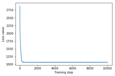
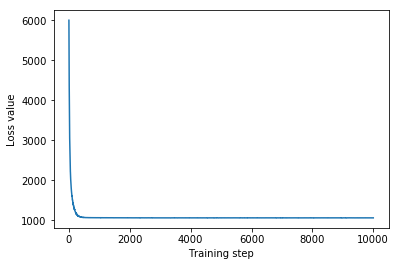
plt.plot(mvn_loss)
plt.xlabel('Training step')
_ = plt.ylabel('Loss value')

Multivariate Normal surrogate posterior ELBO: -1065.705322265625

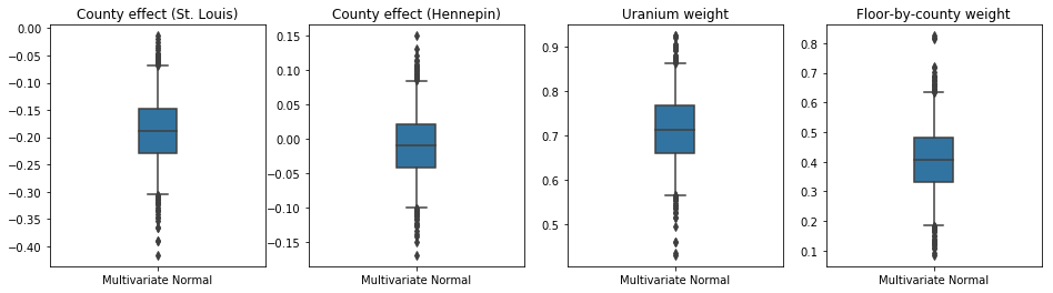
เนื่องจากตัวแทนหลังที่ผ่านการฝึกอบรมเป็นการแจกแจง TFP เราจึงสามารถนำตัวอย่างจากตัวอย่างนั้นและประมวลผลเพื่อสร้างช่วงหลังที่น่าเชื่อถือสำหรับพารามิเตอร์

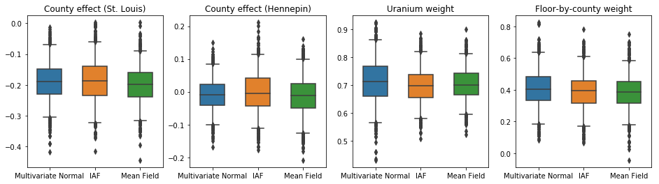
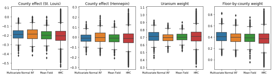
กล่องและเคราแปลงด้านล่างจะแสดง 50% และ 95% ช่วงเวลาที่น่าเชื่อถือ สำหรับผลเขตของสองมณฑลที่ใหญ่ที่สุดและน้ำหนักถดถอยวัดยูเรเนียมดินและพื้นเฉลี่ยโดยมณฑล ช่วงหลังที่น่าเชื่อถือสำหรับผลกระทบของเคาน์ตีบ่งชี้ว่าที่ตั้งในเขตเซนต์หลุยส์มีความเกี่ยวข้องกับระดับเรดอนที่ต่ำกว่า หลังจากพิจารณาตัวแปรอื่นๆ และผลกระทบของตำแหน่งในเคาน์ตีเฮนเนพินนั้นใกล้จะเป็นกลาง

ช่วงหลังที่น่าเชื่อถือของตุ้มน้ำหนักการถดถอยแสดงให้เห็นว่าระดับยูเรเนียมในดินที่สูงขึ้นมีความสัมพันธ์กับระดับเรดอนที่สูงขึ้น และเขตที่มีการตรวจวัดบนชั้นที่สูงขึ้น (อาจเป็นเพราะบ้านไม่มีชั้นใต้ดิน) มักจะมีระดับเรดอนสูงกว่า ซึ่งอาจเกี่ยวข้องกับคุณสมบัติของดินและผลกระทบต่อประเภทของโครงสร้างที่สร้างขึ้น

ค่าสัมประสิทธิ์ของพื้น (ที่กำหนดขึ้นเอง) เป็นค่าลบ ซึ่งบ่งชี้ว่าชั้นล่างมีระดับเรดอนสูงกว่าที่คาดไว้

st_louis_co = 69  # Index of St. Louis, the county with the most observations.
hennepin_co = 25  # Index of Hennepin, with the second-most observations.

def pack_samples(samples):
  return {'County effect (St. Louis)': samples.county_effect[..., st_louis_co],
          'County effect (Hennepin)': samples.county_effect[..., hennepin_co],
          'Uranium weight': samples.uranium_weight,
          'Floor-by-county weight': samples.county_floor_weight}

def plot_boxplot(posterior_samples):
  fig, axes = plt.subplots(1, 4, figsize=(16, 4))

  # Invert the results dict for easier plotting.
  k = list(posterior_samples.values())[0].keys()
  plot_results = {
      v: {p: posterior_samples[p][v] for p in posterior_samples} for v in k}
  for i, (var, var_results) in enumerate(plot_results.items()):
    sns.boxplot(data=list(var_results.values()), ax=axes[i],
                width=0.18*len(var_results), whis=(2.5, 97.5))
    # axes[i].boxplot(list(var_results.values()), whis=(2.5, 97.5))
    axes[i].title.set_text(var)
    fs = 10 if len(var_results) < 4 else 8
    axes[i].set_xticklabels(list(var_results.keys()), fontsize=fs)

results = {'Multivariate Normal': pack_samples(mvn_samples)}

print('Bias is: {:.2f}'.format(bias.numpy()))
print('Floor fixed effect is: {:.2f}'.format(floor_weight.numpy()))
plot_boxplot(results)

Bias is: 1.40
Floor fixed effect is: -0.72

Inverse Autoregressive Flow ตัวแทนหลัง

Inverse Autoregressive Flows (IAFs) เป็นกระแสที่ทำให้เป็นมาตรฐานซึ่งใช้โครงข่ายประสาทเทียมเพื่อจับภาพการพึ่งพาที่ซับซ้อนและไม่เชิงเส้นระหว่างส่วนประกอบของการกระจาย ต่อไป เราสร้างตัวแทนเสมือนด้านหลังเพื่อดูว่าโมเดลที่มีความจุสูงกว่าและปรับเปลี่ยนได้ดีกว่านี้มีประสิทธิภาพเหนือกว่าตัวแปรหลายตัวแปรที่มีข้อจำกัด Normal หรือไม่

# Build a standard Normal with a vector `event_shape`, with length equal to the
# total number of degrees of freedom in the posterior.
base_distribution = tfd.Sample(
    tfd.Normal(0., 1.), sample_shape=[tf.reduce_sum(flat_event_size)])

# Apply an IAF to the base distribution.
num_iafs = 2
iaf_bijectors = [
    tfb.Invert(tfb.MaskedAutoregressiveFlow(
        shift_and_log_scale_fn=tfb.AutoregressiveNetwork(
            params=2, hidden_units=[256, 256], activation='relu')))
    for _ in range(num_iafs)
]

# Split the base distribution's `event_shape` into components that are equal
# in size to the prior's components.
split = tfb.Split(flat_event_size)

# Chain these bijectors and apply them to the standard Normal base distribution
# to build the surrogate posterior. `event_space_bijector`,
# `unflatten_bijector`, and `reshape_bijector` are the same as in the
# multivariate Normal surrogate posterior.
iaf_surrogate_posterior = tfd.TransformedDistribution(
    base_distribution,
    bijector=tfb.Chain([
         event_space_bijector,  # constrain the surrogate to the support of the prior
         unflatten_bijector,  # pack the reshaped components into the `event_shape` structure of the prior
         reshape_bijector,  # reshape the vector-valued components to match the shapes of the prior components
         split] +  # Split the samples into components of the same size as the prior components
         iaf_bijectors  # Apply a flow model to the Tensor-valued standard Normal distribution
         ))

ฝึกตัวแทน IAF หลัง

optimizer=tf.optimizers.Adam(learning_rate=1e-2)
iaf_loss = tfp.vi.fit_surrogate_posterior(
  target_model.unnormalized_log_prob,
  iaf_surrogate_posterior,
  optimizer=optimizer,
  num_steps=10**4,
  sample_size=4,
  jit_compile=True)

iaf_samples = iaf_surrogate_posterior.sample(1000)
iaf_final_elbo = tf.reduce_mean(
    target_model.unnormalized_log_prob(*iaf_samples)
    - iaf_surrogate_posterior.log_prob(iaf_samples))
print('IAF surrogate posterior ELBO: {}'.format(iaf_final_elbo))

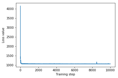
plt.plot(iaf_loss)
plt.xlabel('Training step')
_ = plt.ylabel('Loss value')

IAF surrogate posterior ELBO: -1065.3663330078125

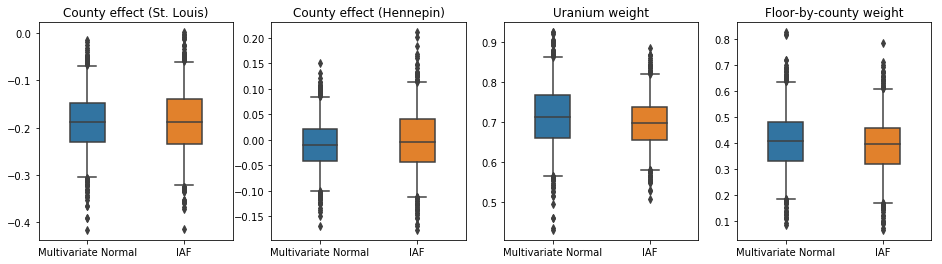
ช่วงที่น่าเชื่อถือสำหรับหลังตัวแทน IAF นั้นคล้ายคลึงกับช่วงปกติที่มีหลายตัวแปรที่มีข้อจำกัด

results['IAF'] = pack_samples(iaf_samples)
plot_boxplot(results)

พื้นฐาน: หลังตัวแทนเสมือนสนามกลาง

VI ตัวแทนหลังมักจะถูกสันนิษฐานว่าเป็นค่าเฉลี่ยฟิลด์ (อิสระ) การแจกแจงแบบปกติด้วยค่าเฉลี่ยและความแปรปรวนที่ฝึกได้ซึ่งถูก จำกัด ให้สนับสนุนก่อนหน้านี้ด้วยการเปลี่ยนแปลงแบบสองทาง เรากำหนดส่วนหลังของตัวแทนเสมือนที่มีฟิลด์กลางเพิ่มเติมจากส่วนหลังของตัวแทนเสมือนที่แสดงอารมณ์อีกสองคน โดยใช้สูตรทั่วไปเดียวกันกับส่วนหลังของตัวแทนเสมือนหลายตัวแปร

# A block-diagonal linear operator, in which each block is a diagonal operator,
# transforms the standard Normal base distribution to produce a mean-field
# surrogate posterior.
operators = (tf.linalg.LinearOperatorDiag,
             tf.linalg.LinearOperatorDiag,
             tf.linalg.LinearOperatorDiag)
block_diag_linop = (
    tfp.experimental.vi.util.build_trainable_linear_operator_block(
        operators, flat_event_size))
mean_field_scale = tfb.ScaleMatvecLinearOperatorBlock(block_diag_linop)

mean_field_loc = tfb.JointMap(
    tf.nest.map_structure(
        lambda s: tfb.Shift(
            tf.Variable(tf.random.uniform(
                (s,), minval=-2., maxval=2., dtype=tf.float32))),
        flat_event_size))

mean_field_surrogate_posterior = tfd.TransformedDistribution(
    base_standard_dist,
    bijector = tfb.Chain(  # Note that the chained bijectors are applied in reverse order
        [
         event_space_bijector,  # constrain the surrogate to the support of the prior
         unflatten_bijector,  # pack the reshaped components into the `event_shape` structure of the posterior
         reshape_bijector, # reshape the vector-valued components to match the shapes of the posterior components
         mean_field_loc,   # allow for nonzero mean
         mean_field_scale  # apply the block matrix transformation to the standard Normal distribution
         ]))

optimizer=tf.optimizers.Adam(learning_rate=1e-2)
mean_field_loss = tfp.vi.fit_surrogate_posterior(
    target_model.unnormalized_log_prob,
    mean_field_surrogate_posterior,
    optimizer=optimizer,
    num_steps=10**4,
    sample_size=16,
    jit_compile=True)

mean_field_samples = mean_field_surrogate_posterior.sample(1000)
mean_field_final_elbo = tf.reduce_mean(
    target_model.unnormalized_log_prob(*mean_field_samples)
    - mean_field_surrogate_posterior.log_prob(mean_field_samples))
print('Mean-field surrogate posterior ELBO: {}'.format(mean_field_final_elbo))

plt.plot(mean_field_loss)
plt.xlabel('Training step')
_ = plt.ylabel('Loss value')

Mean-field surrogate posterior ELBO: -1065.7652587890625

ในกรณีนี้ ค่าเฉลี่ยหลังตัวแทนภาคสนามจะให้ผลลัพธ์ที่คล้ายคลึงกันกับกลุ่มหลังตัวแทนที่แสดงออกมากขึ้น ซึ่งบ่งชี้ว่าแบบจำลองที่เรียบง่ายกว่านี้อาจเพียงพอสำหรับงานอนุมาน

results['Mean Field'] = pack_samples(mean_field_samples)
plot_boxplot(results)

ความจริงพื้นฐาน: Hamiltonian Monte Carlo (HMC)

เราใช้ HMC เพื่อสร้างตัวอย่าง "ความจริงพื้นฐาน" จากส่วนหลังที่แท้จริง เพื่อเปรียบเทียบกับผลลัพธ์ของตัวแทนส่วนหลัง

num_chains = 8
num_leapfrog_steps = 3
step_size = 0.4
num_steps=20000

flat_event_shape = tf.nest.flatten(target_model.event_shape)
enum_components = list(range(len(flat_event_shape)))
bijector = tfb.Restructure(
    enum_components,
    tf.nest.pack_sequence_as(target_model.event_shape, enum_components))(
        target_model.experimental_default_event_space_bijector())

current_state = bijector(
    tf.nest.map_structure(
        lambda e: tf.zeros([num_chains] + list(e), dtype=tf.float32),
    target_model.event_shape))

hmc = tfp.mcmc.HamiltonianMonteCarlo(
    target_log_prob_fn=target_model.unnormalized_log_prob,
    num_leapfrog_steps=num_leapfrog_steps,
    step_size=[tf.fill(s.shape, step_size) for s in current_state])

hmc = tfp.mcmc.TransformedTransitionKernel(
    hmc, bijector)
hmc = tfp.mcmc.DualAveragingStepSizeAdaptation(
    hmc,
    num_adaptation_steps=int(num_steps // 2 * 0.8),
    target_accept_prob=0.9)

chain, is_accepted = tf.function(
    lambda current_state: tfp.mcmc.sample_chain(
        current_state=current_state,
        kernel=hmc,
        num_results=num_steps // 2,
        num_burnin_steps=num_steps // 2,
        trace_fn=lambda _, pkr:
        (pkr.inner_results.inner_results.is_accepted),
        ),
    autograph=False,
    jit_compile=True)(current_state)

accept_rate = tf.reduce_mean(tf.cast(is_accepted, tf.float32))
ess = tf.nest.map_structure(
    lambda c: tfp.mcmc.effective_sample_size(
        c,
        cross_chain_dims=1,
        filter_beyond_positive_pairs=True),
    chain)

r_hat = tf.nest.map_structure(tfp.mcmc.potential_scale_reduction, chain)
hmc_samples = pack_samples(
    tf.nest.pack_sequence_as(target_model.event_shape, chain))
print('Acceptance rate is {}'.format(accept_rate))

Acceptance rate is 0.9008625149726868

พล็อตการติดตามตัวอย่างไปยังผลลัพธ์ HMC ของการตรวจสุขภาพจิต

def plot_traces(var_name, samples):
  fig, axes = plt.subplots(1, 2, figsize=(14, 1.5), sharex='col', sharey='col')
  for chain in range(num_chains):
    s = samples.numpy()[:, chain]
    axes[0].plot(s, alpha=0.7)
    sns.kdeplot(s, ax=axes[1], shade=False)
    axes[0].title.set_text("'{}' trace".format(var_name))
    axes[1].title.set_text("'{}' distribution".format(var_name))
    axes[0].set_xlabel('Iteration')

warnings.filterwarnings('ignore')
for var, var_samples in hmc_samples.items():
  plot_traces(var, var_samples)

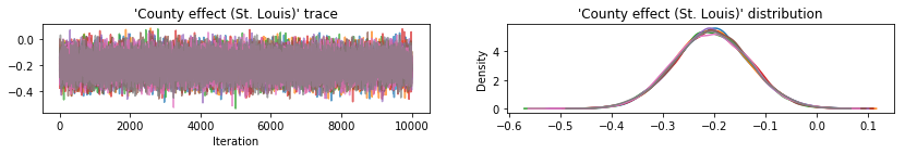
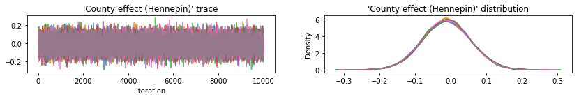
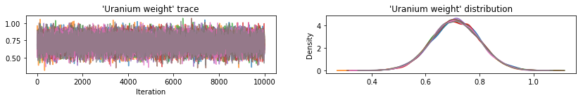
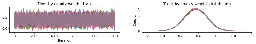
ตัวแทนหลังทั้งสามสร้างช่วงเวลาที่น่าเชื่อถือซึ่งมองเห็นได้คล้ายกับตัวอย่าง HMC แม้ว่าบางครั้งอาจกระจายไม่ทั่วถึงเนื่องจากผลกระทบของการสูญเสีย ELBO ตามปกติใน VI

results['HMC'] = hmc_samples
plot_boxplot(results)

ผลลัพธ์เพิ่มเติม

ฟังก์ชันพล็อต

plt.rcParams.update({'axes.titlesize': 'medium', 'xtick.labelsize': 'medium'})
def plot_loss_and_elbo():
  fig, axes = plt.subplots(1, 2, figsize=(12, 4))

  axes[0].scatter([0, 1, 2],
                  [mvn_final_elbo.numpy(),
                  iaf_final_elbo.numpy(),
                  mean_field_final_elbo.numpy()])
  axes[0].set_xticks(ticks=[0, 1, 2])
  axes[0].set_xticklabels(labels=[
    'Multivariate Normal', 'IAF', 'Mean Field'])
  axes[0].title.set_text('Evidence Lower Bound (ELBO)')

  axes[1].plot(mvn_loss, label='Multivariate Normal')
  axes[1].plot(iaf_loss, label='IAF')
  axes[1].plot(mean_field_loss, label='Mean Field')
  axes[1].set_ylim([1000, 4000])
  axes[1].set_xlabel('Training step')
  axes[1].set_ylabel('Loss (negative ELBO)')
  axes[1].title.set_text('Loss')
  plt.legend()
  plt.show()

plt.rcParams.update({'axes.titlesize': 'medium', 'xtick.labelsize': 'small'})
def plot_kdes(num_chains=8):
  fig, axes = plt.subplots(2, 2, figsize=(12, 8))
  k = list(results.values())[0].keys()
  plot_results = {
      v: {p: results[p][v] for p in results} for v in k}
  for i, (var, var_results) in enumerate(plot_results.items()):
    ax = axes[i % 2, i // 2]
    for posterior, posterior_results in var_results.items():
      if posterior == 'HMC':
        label = posterior
        for chain in range(num_chains):
          sns.kdeplot(
              posterior_results[:, chain],
              ax=ax, shade=False, color='k', linestyle=':', label=label)
          label=None
      else:
        sns.kdeplot(
            posterior_results, ax=ax, shade=False, label=posterior)
        ax.title.set_text('{}'.format(var))
    ax.legend()

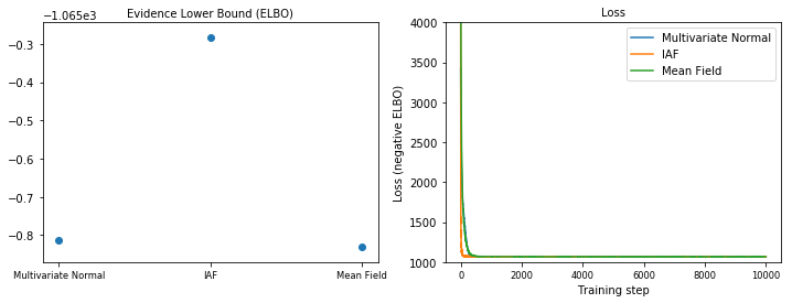
หลักฐานขอบเขตล่าง (ELBO)

IAF ซึ่งเป็นกลุ่มหลังตัวแทนที่ใหญ่ที่สุดและยืดหยุ่นที่สุด มาบรรจบกันที่ขอบเขตล่างสุดของหลักฐาน (ELBO)

plot_loss_and_elbo()

ตัวอย่างหลัง

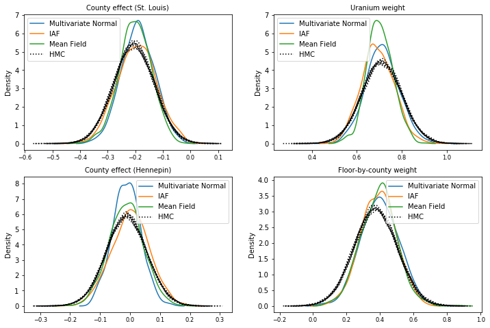
ตัวอย่างจากตัวแทนหลังแต่ละคน เปรียบเทียบกับตัวอย่างความจริงภาคพื้นดินของ HMC (การแสดงภาพตัวอย่างที่แสดงในแผนภาพกล่องที่ต่างกัน)

plot_kdes()

บทสรุป

ใน Colab นี้ เราสร้าง VI ตัวแทนหลังโดยใช้การแจกแจงร่วมและ bijectors แบบหลายส่วน และปรับให้เหมาะสมเพื่อประมาณช่วงเวลาที่น่าเชื่อถือสำหรับน้ำหนักในแบบจำลองการถดถอยบนชุดข้อมูลเรดอน สำหรับโมเดลที่เรียบง่ายนี้ ตัวแทนหลังที่แสดงอารมณ์ได้ชัดเจนกว่าจะแสดงในลักษณะเดียวกับหลังตัวแทนตัวแทนที่มีใจกว้าง อย่างไรก็ตาม เครื่องมือที่เราสาธิตสามารถใช้เพื่อสร้างส่วนหลังของตัวแทนเสมือนที่ยืดหยุ่นได้หลากหลาย ซึ่งเหมาะสำหรับโมเดลที่ซับซ้อนมากขึ้น