
| | |  ดูแหล่งที่มาบน GitHub ดูแหล่งที่มาบน GitHub | |
บทช่วยสอนนี้จะสำรวจอัลกอริธึมการคำนวณการไล่ระดับสีสำหรับค่าความคาดหวังของวงจรควอนตัม
การคำนวณความลาดชันของค่าคาดหวังของสิ่งที่สังเกตได้บางอย่างในวงจรควอนตัมเป็นกระบวนการที่เกี่ยวข้อง ค่าความคาดหวังของสิ่งที่สังเกตได้นั้นไม่มีความหรูหราในการมีสูตรการไล่ระดับสีเชิงวิเคราะห์ที่เขียนง่ายเสมอ ซึ่งต่างจากการแปลงการเรียนรู้ของเครื่องแบบดั้งเดิม เช่น การคูณเมทริกซ์หรือการบวกเวกเตอร์ที่มีสูตรการไล่ระดับสีเชิงวิเคราะห์ซึ่งเขียนได้ง่าย ด้วยเหตุนี้ จึงมีวิธีการคำนวณการไล่ระดับควอนตัมที่แตกต่างกันซึ่งสะดวกสำหรับสถานการณ์ต่างๆ บทช่วยสอนนี้จะเปรียบเทียบและเปรียบเทียบรูปแบบการสร้างความแตกต่างที่แตกต่างกันสองแบบ
ติดตั้ง
pip install tensorflow==2.7.0
ติดตั้ง TensorFlow Quantum:
pip install tensorflow-quantum
# Update package resources to account for version changes.
import importlib, pkg_resources
importlib.reload(pkg_resources)
<module 'pkg_resources' from '/tmpfs/src/tf_docs_env/lib/python3.7/site-packages/pkg_resources/__init__.py'>
ตอนนี้นำเข้า TensorFlow และการพึ่งพาโมดูล:
import tensorflow as tf
import tensorflow_quantum as tfq

import cirq
import sympy
import numpy as np

# visualization tools
%matplotlib inline
import matplotlib.pyplot as plt
from cirq.contrib.svg import SVGCircuit
2022-02-04 12:25:24.733670: E tensorflow/stream_executor/cuda/cuda_driver.cc:271] failed call to cuInit: CUDA_ERROR_NO_DEVICE: no CUDA-capable device is detected
1. เบื้องต้น
มาทำให้แนวคิดของการคำนวณเกรเดียนต์สำหรับวงจรควอนตัมมีความเป็นรูปธรรมมากขึ้นกัน สมมติว่าคุณมีวงจรแบบกำหนดพารามิเตอร์ดังนี้:
qubit = cirq.GridQubit(0, 0)
my_circuit = cirq.Circuit(cirq.Y(qubit)**sympy.Symbol('alpha'))
SVGCircuit(my_circuit)
findfont: Font family ['Arial'] not found. Falling back to DejaVu Sans.

พร้อมทั้งสังเกตได้ว่า
pauli_x = cirq.X(qubit)
pauli_x
cirq.X(cirq.GridQubit(0, 0))ตัวยึดตำแหน่ง23
ดูที่โอเปอเรเตอร์นี้ คุณจะรู้ว่า \(⟨Y(\alpha)| X | Y(\alpha)⟩ = \sin(\pi \alpha)\)
def my_expectation(op, alpha):
    """Compute ⟨Y(alpha)| `op` | Y(alpha)⟩"""
    params = {'alpha': alpha}
    sim = cirq.Simulator()
    final_state_vector = sim.simulate(my_circuit, params).final_state_vector
    return op.expectation_from_state_vector(final_state_vector, {qubit: 0}).real


my_alpha = 0.3
print("Expectation=", my_expectation(pauli_x, my_alpha))
print("Sin Formula=", np.sin(np.pi * my_alpha))
Expectation= 0.80901700258255
Sin Formula= 0.8090169943749475
และถ้าคุณกำหนด \(f_{1}(\alpha) = ⟨Y(\alpha)| X | Y(\alpha)⟩\) แล้ว \(f_{1}^{'}(\alpha) = \pi \cos(\pi \alpha)\)มาตรวจสอบสิ่งนี้:
def my_grad(obs, alpha, eps=0.01):
    grad = 0
    f_x = my_expectation(obs, alpha)
    f_x_prime = my_expectation(obs, alpha + eps)
    return ((f_x_prime - f_x) / eps).real


print('Finite difference:', my_grad(pauli_x, my_alpha))
print('Cosine formula:   ', np.pi * np.cos(np.pi * my_alpha))
Finite difference: 1.8063604831695557
Cosine formula:    1.8465818304904567
2. ความจำเป็นในการสร้างความแตกต่าง
ด้วยวงจรขนาดใหญ่ คุณจะไม่โชคดีเสมอไปที่มีสูตรที่คำนวณการไล่ระดับสีของวงจรควอนตัมที่กำหนดได้อย่างแม่นยำ ในกรณีที่สูตรอย่างง่ายไม่เพียงพอในการคำนวณการไล่ระดับสี คลาส tfq.differentiators.Differentiator ช่วยให้คุณสามารถกำหนดอัลกอริทึมสำหรับการคำนวณการไล่ระดับสีของวงจรของคุณได้ ตัวอย่างเช่น คุณสามารถสร้างตัวอย่างด้านบนใหม่ใน TensorFlow Quantum (TFQ) ด้วย:
expectation_calculation = tfq.layers.Expectation(
    differentiator=tfq.differentiators.ForwardDifference(grid_spacing=0.01))

expectation_calculation(my_circuit,
                        operators=pauli_x,
                        symbol_names=['alpha'],
                        symbol_values=[[my_alpha]])
<tf.Tensor: shape=(1, 1), dtype=float32, numpy=array([[0.80901706]], dtype=float32)>
อย่างไรก็ตาม หากคุณเปลี่ยนไปใช้การประมาณการความคาดหวังตามการสุ่มตัวอย่าง (สิ่งที่จะเกิดขึ้นกับอุปกรณ์จริง) ค่าอาจเปลี่ยนแปลงเล็กน้อย ซึ่งหมายความว่าขณะนี้คุณมีค่าประมาณที่ไม่สมบูรณ์:
sampled_expectation_calculation = tfq.layers.SampledExpectation(
    differentiator=tfq.differentiators.ForwardDifference(grid_spacing=0.01))

sampled_expectation_calculation(my_circuit,
                                operators=pauli_x,
                                repetitions=500,
                                symbol_names=['alpha'],
                                symbol_values=[[my_alpha]])
<tf.Tensor: shape=(1, 1), dtype=float32, numpy=array([[0.836]], dtype=float32)>
สิ่งนี้สามารถรวมเป็นปัญหาความแม่นยำที่ร้ายแรงได้อย่างรวดเร็วเมื่อพูดถึงการไล่ระดับสี:
# Make input_points = [batch_size, 1] array.
input_points = np.linspace(0, 5, 200)[:, np.newaxis].astype(np.float32)
exact_outputs = expectation_calculation(my_circuit,
operators=pauli_x,
symbol_names=['alpha'],
symbol_values=input_points)
imperfect_outputs = sampled_expectation_calculation(my_circuit,
operators=pauli_x,
repetitions=500,
symbol_names=['alpha'],
symbol_values=input_points)
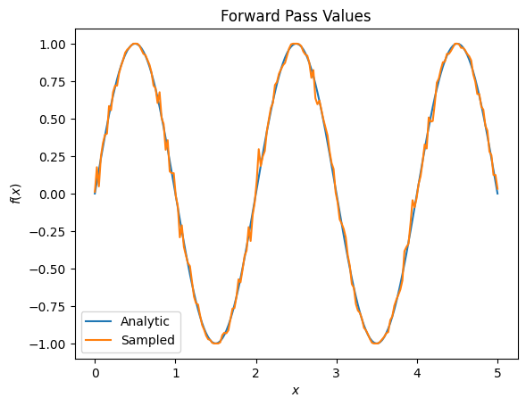
plt.title('Forward Pass Values')
plt.xlabel('$x$')
plt.ylabel('$f(x)$')
plt.plot(input_points, exact_outputs, label='Analytic')
plt.plot(input_points, imperfect_outputs, label='Sampled')
plt.legend()
<matplotlib.legend.Legend at 0x7ff07d556190>ตัวยึดตำแหน่ง33
# Gradients are a much different story.
values_tensor = tf.convert_to_tensor(input_points)

with tf.GradientTape() as g:
    g.watch(values_tensor)
    exact_outputs = expectation_calculation(my_circuit,
                                            operators=pauli_x,
                                            symbol_names=['alpha'],
                                            symbol_values=values_tensor)
analytic_finite_diff_gradients = g.gradient(exact_outputs, values_tensor)

with tf.GradientTape() as g:
    g.watch(values_tensor)
    imperfect_outputs = sampled_expectation_calculation(
        my_circuit,
        operators=pauli_x,
        repetitions=500,
        symbol_names=['alpha'],
        symbol_values=values_tensor)
sampled_finite_diff_gradients = g.gradient(imperfect_outputs, values_tensor)

plt.title('Gradient Values')
plt.xlabel('$x$')
plt.ylabel('$f^{\'}(x)$')
plt.plot(input_points, analytic_finite_diff_gradients, label='Analytic')
plt.plot(input_points, sampled_finite_diff_gradients, label='Sampled')
plt.legend()
<matplotlib.legend.Legend at 0x7ff07adb8dd0>
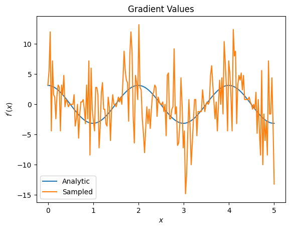
ในที่นี้คุณจะเห็นว่าแม้ว่าสูตรความแตกต่างแบบจำกัดจะคำนวณการไล่ระดับสีอย่างรวดเร็วด้วยตัวมันเองในกรณีเชิงวิเคราะห์ แต่เมื่อกล่าวถึงวิธีการสุ่มตัวอย่างก็มีจุดรบกวนมากเกินไป ต้องใช้เทคนิคอย่างระมัดระวังมากขึ้นเพื่อให้แน่ใจว่าสามารถคำนวณการไล่ระดับสีที่ดีได้ ต่อไป คุณจะดูเทคนิคที่ช้ากว่ามากซึ่งไม่เหมาะสำหรับการคำนวณการไล่ระดับความคาดหวังเชิงวิเคราะห์ แต่จะทำงานได้ดีกว่ามากในกรณีตามตัวอย่างในโลกแห่งความเป็นจริง:
# A smarter differentiation scheme.
gradient_safe_sampled_expectation = tfq.layers.SampledExpectation(
    differentiator=tfq.differentiators.ParameterShift())

with tf.GradientTape() as g:
    g.watch(values_tensor)
    imperfect_outputs = gradient_safe_sampled_expectation(
        my_circuit,
        operators=pauli_x,
        repetitions=500,
        symbol_names=['alpha'],
        symbol_values=values_tensor)

sampled_param_shift_gradients = g.gradient(imperfect_outputs, values_tensor)

plt.title('Gradient Values')
plt.xlabel('$x$')
plt.ylabel('$f^{\'}(x)$')
plt.plot(input_points, analytic_finite_diff_gradients, label='Analytic')
plt.plot(input_points, sampled_param_shift_gradients, label='Sampled')
plt.legend()
<matplotlib.legend.Legend at 0x7ff07ad9ff90>
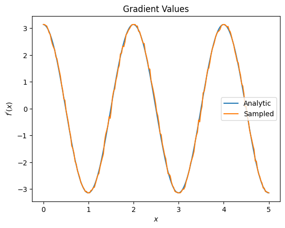
จากด้านบน คุณจะเห็นว่าตัวสร้างความแตกต่างบางตัวเหมาะที่สุดสำหรับสถานการณ์การวิจัยเฉพาะ โดยทั่วไป วิธีการแบบอิงตัวอย่างที่ช้ากว่าซึ่งทนทานต่อสัญญาณรบกวนของอุปกรณ์ ฯลฯ เป็นตัวสร้างความแตกต่างที่ยอดเยี่ยมเมื่อทำการทดสอบหรือใช้อัลกอริทึมในสภาพแวดล้อมที่ "จริง" มากกว่า วิธีการที่เร็วกว่า เช่น ค่าความต่างจำกัดนั้นยอดเยี่ยมสำหรับการคำนวณเชิงวิเคราะห์ และคุณต้องการปริมาณงานที่สูงขึ้น แต่ยังไม่เกี่ยวข้องกับความสามารถในการทำงานของอุปกรณ์ของอัลกอริทึมของคุณ
3. สังเกตได้หลายอย่าง
เรามาแนะนำสิ่งที่สังเกตได้ที่สองกันและดูว่า TensorFlow Quantum รองรับการสังเกตได้หลายรายการสำหรับวงจรเดียวได้อย่างไร
pauli_z = cirq.Z(qubit)
pauli_z
cirq.Z(cirq.GridQubit(0, 0))ตัวยึดตำแหน่ง39
หากสิ่งที่สังเกตได้นี้ใช้กับวงจรเดิม แสดงว่าคุณมี \(f_{2}(\alpha) = ⟨Y(\alpha)| Z | Y(\alpha)⟩ = \cos(\pi \alpha)\) และ \(f_{2}^{'}(\alpha) = -\pi \sin(\pi \alpha)\)ทำการตรวจสอบอย่างรวดเร็ว:
test_value = 0.

print('Finite difference:', my_grad(pauli_z, test_value))
print('Sin formula:      ', -np.pi * np.sin(np.pi * test_value))
Finite difference: -0.04934072494506836
Sin formula:       -0.0
ตัวยึดตำแหน่ง41
เป็นแมตช์ (ใกล้เคียงกัน)
ตอนนี้ถ้าคุณกำหนด \(g(\alpha) = f_{1}(\alpha) + f_{2}(\alpha)\) แล้ว \(g'(\alpha) = f_{1}^{'}(\alpha) + f^{'}_{2}(\alpha)\)การกำหนดมากกว่าหนึ่งสิ่งที่สังเกตได้ใน TensorFlow Quantum เพื่อใช้ร่วมกับวงจรจะเทียบเท่ากับการเพิ่มเงื่อนไขเพิ่มเติมใน \(g\)
ซึ่งหมายความว่าการไล่ระดับของสัญลักษณ์เฉพาะในวงจรจะเท่ากับผลรวมของการไล่ระดับสีโดยคำนึงถึงแต่ละสัญลักษณ์ที่สามารถสังเกตได้ซึ่งนำไปใช้กับวงจรนั้น สิ่งนี้เข้ากันได้กับการไล่ระดับ TensorFlow และการแพร่กระจายย้อนกลับ (โดยที่คุณให้ผลรวมของการไล่ระดับสีเหนือสิ่งที่สังเกตได้ทั้งหมดเป็นการไล่ระดับสีสำหรับสัญลักษณ์เฉพาะ)
sum_of_outputs = tfq.layers.Expectation(
    differentiator=tfq.differentiators.ForwardDifference(grid_spacing=0.01))

sum_of_outputs(my_circuit,
               operators=[pauli_x, pauli_z],
               symbol_names=['alpha'],
               symbol_values=[[test_value]])
<tf.Tensor: shape=(1, 2), dtype=float32, numpy=array([[1.9106855e-15, 1.0000000e+00]], dtype=float32)>ตัวยึดตำแหน่ง43
ที่นี่คุณจะเห็นรายการแรกคือความคาดหวังของ Pauli X และรายการที่สองคือความคาดหวังของ Pauli Z ตอนนี้เมื่อคุณใช้การไล่ระดับสี:
test_value_tensor = tf.convert_to_tensor([[test_value]])

with tf.GradientTape() as g:
    g.watch(test_value_tensor)
    outputs = sum_of_outputs(my_circuit,
                             operators=[pauli_x, pauli_z],
                             symbol_names=['alpha'],
                             symbol_values=test_value_tensor)

sum_of_gradients = g.gradient(outputs, test_value_tensor)

print(my_grad(pauli_x, test_value) + my_grad(pauli_z, test_value))
print(sum_of_gradients.numpy())
3.0917350202798843
[[3.0917213]]
ที่นี่คุณได้ตรวจสอบแล้วว่าผลรวมของการไล่ระดับสีสำหรับแต่ละรายการที่สังเกตได้นั้นเป็นความลาดชันของ \(\alpha\)ลักษณะการทำงานนี้ได้รับการสนับสนุนโดยตัวสร้างความแตกต่างของ TensorFlow Quantum และมีบทบาทสำคัญในความเข้ากันได้กับส่วนที่เหลือของ TensorFlow
4. การใช้งานขั้นสูง
ตัวสร้างความแตกต่างทั้งหมดที่มีอยู่ในคลาสย่อย TensorFlow Quantum tfq.differentiators.Differentiator ในการใช้ตัวสร้างความแตกต่าง ผู้ใช้ต้องใช้อินเทอร์เฟซอย่างใดอย่างหนึ่งจากสองอินเทอร์เฟซ มาตรฐานคือการใช้ get_gradient_circuits ซึ่งบอกคลาสฐานว่าวงจรใดที่จะวัดเพื่อให้ได้ค่าประมาณการไล่ระดับสี หรือคุณสามารถโอเวอร์โหลด differentiate_analytic และ differentiate_sampled ; คลาส tfq.differentiators.Adjoint ใช้เส้นทางนี้
ข้อมูลต่อไปนี้ใช้ TensorFlow Quantum เพื่อนำการไล่ระดับของวงจรไปใช้ คุณจะใช้ตัวอย่างเล็กๆ ของการเปลี่ยนพารามิเตอร์
จำวงจรที่คุณกำหนดไว้ข้างต้น \(|\alpha⟩ = Y^{\alpha}|0⟩\). เช่นเคย คุณสามารถกำหนดฟังก์ชันเป็นค่าคาดหวังของวงจรนี้เทียบกับ \(X\) สังเกตได้ \(f(\alpha) = ⟨\alpha|X|\alpha⟩\)การใช้ กฎการเปลี่ยนพารามิเตอร์ สำหรับวงจรนี้ คุณจะพบว่าอนุพันธ์คือ
\[\frac{\partial}{\partial \alpha} f(\alpha) = \frac{\pi}{2} f\left(\alpha + \frac{1}{2}\right) - \frac{ \pi}{2} f\left(\alpha - \frac{1}{2}\right)\]
ฟังก์ชัน get_gradient_circuits ส่งคืนส่วนประกอบของอนุพันธ์นี้
class MyDifferentiator(tfq.differentiators.Differentiator):
    """A Toy differentiator for <Y^alpha | X |Y^alpha>."""

    def __init__(self):
        pass

    def get_gradient_circuits(self, programs, symbol_names, symbol_values):
        """Return circuits to compute gradients for given forward pass circuits.

        Every gradient on a quantum computer can be computed via measurements
        of transformed quantum circuits.  Here, you implement a custom gradient
        for a specific circuit.  For a real differentiator, you will need to
        implement this function in a more general way.  See the differentiator
        implementations in the TFQ library for examples.
        """

        # The two terms in the derivative are the same circuit...
        batch_programs = tf.stack([programs, programs], axis=1)

        # ... with shifted parameter values.
        shift = tf.constant(1/2)
        forward = symbol_values + shift
        backward = symbol_values - shift
        batch_symbol_values = tf.stack([forward, backward], axis=1)

        # Weights are the coefficients of the terms in the derivative.
        num_program_copies = tf.shape(batch_programs)[0]
        batch_weights = tf.tile(tf.constant([[[np.pi/2, -np.pi/2]]]),
                                [num_program_copies, 1, 1])

        # The index map simply says which weights go with which circuits.
        batch_mapper = tf.tile(
            tf.constant([[[0, 1]]]), [num_program_copies, 1, 1])

        return (batch_programs, symbol_names, batch_symbol_values,
                batch_weights, batch_mapper)
คลาสฐาน Differentiator ใช้ส่วนประกอบที่ส่งคืนจาก get_gradient_circuits เพื่อคำนวณอนุพันธ์ ดังในสูตรการเปลี่ยนพารามิเตอร์ที่คุณเห็นด้านบน ตัวสร้างความแตกต่างใหม่นี้สามารถใช้ได้กับวัตถุ tfq.layer ที่มีอยู่:
custom_dif = MyDifferentiator()
custom_grad_expectation = tfq.layers.Expectation(differentiator=custom_dif)

# Now let's get the gradients with finite diff.
with tf.GradientTape() as g:
    g.watch(values_tensor)
    exact_outputs = expectation_calculation(my_circuit,
                                            operators=[pauli_x],
                                            symbol_names=['alpha'],
                                            symbol_values=values_tensor)

analytic_finite_diff_gradients = g.gradient(exact_outputs, values_tensor)

# Now let's get the gradients with custom diff.
with tf.GradientTape() as g:
    g.watch(values_tensor)
    my_outputs = custom_grad_expectation(my_circuit,
                                         operators=[pauli_x],
                                         symbol_names=['alpha'],
                                         symbol_values=values_tensor)

my_gradients = g.gradient(my_outputs, values_tensor)

plt.subplot(1, 2, 1)
plt.title('Exact Gradient')
plt.plot(input_points, analytic_finite_diff_gradients.numpy())
plt.xlabel('x')
plt.ylabel('f(x)')
plt.subplot(1, 2, 2)
plt.title('My Gradient')
plt.plot(input_points, my_gradients.numpy())
plt.xlabel('x')
Text(0.5, 0, 'x')
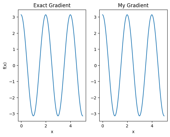
ขณะนี้สามารถใช้ตัวสร้างความแตกต่างใหม่เพื่อสร้างความแตกต่างได้
# Create a noisy sample based expectation op.
expectation_sampled = tfq.get_sampled_expectation_op(
    cirq.DensityMatrixSimulator(noise=cirq.depolarize(0.01)))

# Make it differentiable with your differentiator:
# Remember to refresh the differentiator before attaching the new op
custom_dif.refresh()
differentiable_op = custom_dif.generate_differentiable_op(
    sampled_op=expectation_sampled)

# Prep op inputs.
circuit_tensor = tfq.convert_to_tensor([my_circuit])
op_tensor = tfq.convert_to_tensor([[pauli_x]])
single_value = tf.convert_to_tensor([[my_alpha]])
num_samples_tensor = tf.convert_to_tensor([[5000]])

with tf.GradientTape() as g:
    g.watch(single_value)
    forward_output = differentiable_op(circuit_tensor, ['alpha'], single_value,
                                       op_tensor, num_samples_tensor)

my_gradients = g.gradient(forward_output, single_value)

print('---TFQ---')
print('Foward:  ', forward_output.numpy())
print('Gradient:', my_gradients.numpy())
print('---Original---')
print('Forward: ', my_expectation(pauli_x, my_alpha))
print('Gradient:', my_grad(pauli_x, my_alpha))
---TFQ---
Foward:   [[0.8016]]
Gradient: [[1.7932211]]
---Original---
Forward:  0.80901700258255
Gradient: 1.8063604831695557