
| | |  ดูแหล่งที่มาบน GitHub ดูแหล่งที่มาบน GitHub | |
บทช่วยสอนนี้สร้างเครือข่ายนิวรัลควอนตัม (QNN) เพื่อจำแนก MNIST เวอร์ชันที่เรียบง่าย ซึ่งคล้ายกับแนวทางที่ใช้ใน Farhi et al ประสิทธิภาพของโครงข่ายประสาทควอนตัมในปัญหาข้อมูลแบบคลาสสิกนี้ เปรียบเทียบกับโครงข่ายประสาทเทียมแบบคลาสสิก
ติดตั้ง
pip install tensorflow==2.7.0
ติดตั้ง TensorFlow Quantum:
pip install tensorflow-quantum
# Update package resources to account for version changes.
import importlib, pkg_resources
importlib.reload(pkg_resources)
<module 'pkg_resources' from '/tmpfs/src/tf_docs_env/lib/python3.7/site-packages/pkg_resources/__init__.py'>
ตอนนี้นำเข้า TensorFlow และการพึ่งพาโมดูล:
import tensorflow as tf
import tensorflow_quantum as tfq

import cirq
import sympy
import numpy as np
import seaborn as sns
import collections

# visualization tools
%matplotlib inline
import matplotlib.pyplot as plt
from cirq.contrib.svg import SVGCircuit
2022-02-04 12:29:39.759643: E tensorflow/stream_executor/cuda/cuda_driver.cc:271] failed call to cuInit: CUDA_ERROR_NO_DEVICE: no CUDA-capable device is detected
1. โหลดข้อมูล
ในบทช่วยสอนนี้ คุณจะสร้างตัวแยกประเภทไบนารีเพื่อแยกความแตกต่างระหว่างตัวเลข 3 และ 6 ตาม Farhi et al ส่วนนี้ครอบคลุมถึงการจัดการข้อมูลที่:
- โหลดข้อมูลดิบจาก Keras
- กรองชุดข้อมูลให้เหลือเพียง 3s และ 6s
- ลดขนาดรูปภาพเพื่อให้พอดีกับคอมพิวเตอร์ควอนตัม
- ลบตัวอย่างที่ขัดแย้ง
- แปลงภาพไบนารีเป็นวงจร Cirq
- แปลงวงจร Cirq เป็นวงจรควอนตัม TensorFlow
1.1 โหลดข้อมูลดิบ
โหลดชุดข้อมูล MNIST ที่แจกจ่ายด้วย Keras
(x_train, y_train), (x_test, y_test) = tf.keras.datasets.mnist.load_data()

# Rescale the images from [0,255] to the [0.0,1.0] range.
x_train, x_test = x_train[..., np.newaxis]/255.0, x_test[..., np.newaxis]/255.0

print("Number of original training examples:", len(x_train))
print("Number of original test examples:", len(x_test))
Downloading data from https://storage.googleapis.com/tensorflow/tf-keras-datasets/mnist.npz
11493376/11490434 [==============================] - 0s 0us/step
11501568/11490434 [==============================] - 0s 0us/step
Number of original training examples: 60000
Number of original test examples: 10000
กรองชุดข้อมูลเพื่อเก็บเฉพาะ 3s และ 6s ลบคลาสอื่น ในเวลาเดียวกันให้แปลงป้ายกำกับ y เป็นบูลีน: True สำหรับ 3 และ False สำหรับ 6
def filter_36(x, y):
    keep = (y == 3) | (y == 6)
    x, y = x[keep], y[keep]
    y = y == 3
    return x,y
x_train, y_train = filter_36(x_train, y_train)
x_test, y_test = filter_36(x_test, y_test)

print("Number of filtered training examples:", len(x_train))
print("Number of filtered test examples:", len(x_test))
Number of filtered training examples: 12049
Number of filtered test examples: 1968
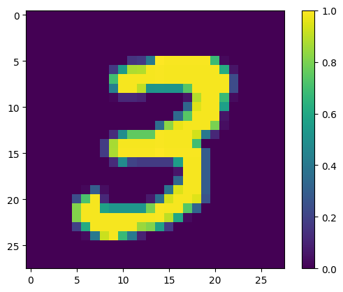
แสดงตัวอย่างแรก:
print(y_train[0])

plt.imshow(x_train[0, :, :, 0])
plt.colorbar()
True
<matplotlib.colorbar.Colorbar at 0x7fac6ad4bd90>
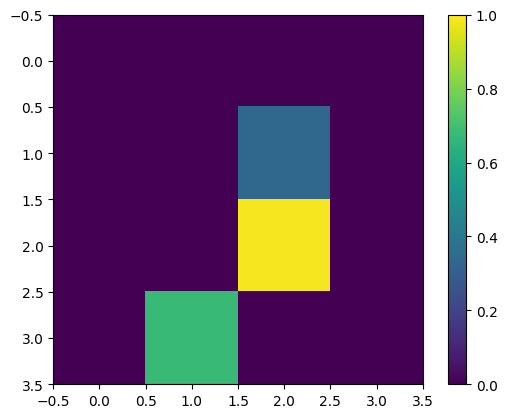
1.2 ลดขนาดภาพ
ขนาดรูปภาพ 28x28 ใหญ่เกินไปสำหรับคอมพิวเตอร์ควอนตัมปัจจุบัน ปรับขนาดภาพลงเป็น 4x4:
x_train_small = tf.image.resize(x_train, (4,4)).numpy()
x_test_small = tf.image.resize(x_test, (4,4)).numpy()
อีกครั้ง แสดงตัวอย่างการฝึกครั้งแรก—หลังจากปรับขนาด:
print(y_train[0])

plt.imshow(x_train_small[0,:,:,0], vmin=0, vmax=1)
plt.colorbar()
True
<matplotlib.colorbar.Colorbar at 0x7fabf807fe10>
1.3 ลบตัวอย่างที่ขัดแย้ง
จากส่วนที่ 3.3 การเรียนรู้เพื่อแยกแยะตัวเลข ของ Farhi et al. ให้กรองชุดข้อมูลเพื่อลบภาพที่ระบุว่าเป็นของทั้งสองคลาส
นี่ไม่ใช่ขั้นตอนการเรียนรู้ด้วยเครื่องมาตรฐาน แต่รวมอยู่ในความสนใจในการติดตามบทความนี้
def remove_contradicting(xs, ys):
    mapping = collections.defaultdict(set)
    orig_x = {}
    # Determine the set of labels for each unique image:
    for x,y in zip(xs,ys):
       orig_x[tuple(x.flatten())] = x
       mapping[tuple(x.flatten())].add(y)

    new_x = []
    new_y = []
    for flatten_x in mapping:
      x = orig_x[flatten_x]
      labels = mapping[flatten_x]
      if len(labels) == 1:
          new_x.append(x)
          new_y.append(next(iter(labels)))
      else:
          # Throw out images that match more than one label.
          pass

    num_uniq_3 = sum(1 for value in mapping.values() if len(value) == 1 and True in value)
    num_uniq_6 = sum(1 for value in mapping.values() if len(value) == 1 and False in value)
    num_uniq_both = sum(1 for value in mapping.values() if len(value) == 2)

    print("Number of unique images:", len(mapping.values()))
    print("Number of unique 3s: ", num_uniq_3)
    print("Number of unique 6s: ", num_uniq_6)
    print("Number of unique contradicting labels (both 3 and 6): ", num_uniq_both)
    print()
    print("Initial number of images: ", len(xs))
    print("Remaining non-contradicting unique images: ", len(new_x))

    return np.array(new_x), np.array(new_y)
จำนวนผลลัพธ์ไม่ตรงกับค่าที่รายงานอย่างใกล้ชิด แต่ไม่ได้ระบุขั้นตอนที่แน่นอน
นอกจากนี้ ยังควรสังเกตด้วยว่าการใช้ตัวอย่างการกรองที่ขัดแย้ง ณ จุดนี้ไม่ได้ป้องกันโมเดลจากการรับตัวอย่างการฝึกที่ขัดแย้งโดยสิ้นเชิง: ขั้นตอนต่อไปจะเป็นการรวมข้อมูลสองส่วนซึ่งจะทำให้เกิดการชนกันมากขึ้น
x_train_nocon, y_train_nocon = remove_contradicting(x_train_small, y_train)
Number of unique images: 10387
Number of unique 3s:  4912
Number of unique 6s:  5426
Number of unique contradicting labels (both 3 and 6):  49

Initial number of images:  12049
Remaining non-contradicting unique images:  10338
1.4 เข้ารหัสข้อมูลเป็นวงจรควอนตัม
ในการประมวลผลภาพโดยใช้คอมพิวเตอร์ควอนตัม Farhi et al. เสนอให้แสดงแต่ละพิกเซลด้วย qubit โดยมีสถานะขึ้นอยู่กับค่าของพิกเซล ขั้นตอนแรกคือการแปลงเป็นการเข้ารหัสไบนารี
THRESHOLD = 0.5

x_train_bin = np.array(x_train_nocon > THRESHOLD, dtype=np.float32)
x_test_bin = np.array(x_test_small > THRESHOLD, dtype=np.float32)
หากคุณต้องลบภาพที่ขัดแย้ง ณ จุดนี้ คุณจะเหลือเพียง 193 ซึ่งไม่น่าจะเพียงพอสำหรับการฝึกอบรมที่มีประสิทธิภาพ
_ = remove_contradicting(x_train_bin, y_train_nocon)
Number of unique images: 193
Number of unique 3s:  80
Number of unique 6s:  69
Number of unique contradicting labels (both 3 and 6):  44

Initial number of images:  10338
Remaining non-contradicting unique images:  149
ตัวยึดตำแหน่ง23
qubits ที่ดัชนีพิกเซลที่มีค่าที่เกินขีดจำกัด จะถูกหมุนผ่านเกท \(X\)
def convert_to_circuit(image):
    """Encode truncated classical image into quantum datapoint."""
    values = np.ndarray.flatten(image)
    qubits = cirq.GridQubit.rect(4, 4)
    circuit = cirq.Circuit()
    for i, value in enumerate(values):
        if value:
            circuit.append(cirq.X(qubits[i]))
    return circuit


x_train_circ = [convert_to_circuit(x) for x in x_train_bin]
x_test_circ = [convert_to_circuit(x) for x in x_test_bin]
นี่คือวงจรที่สร้างขึ้นสำหรับตัวอย่างแรก (แผนภาพวงจรไม่แสดง qubits ที่มีประตูเป็นศูนย์):
SVGCircuit(x_train_circ[0])
findfont: Font family ['Arial'] not found. Falling back to DejaVu Sans.

เปรียบเทียบวงจรนี้กับดัชนีที่ค่าภาพเกินเกณฑ์:
bin_img = x_train_bin[0,:,:,0]
indices = np.array(np.where(bin_img)).T
indices
array([[2, 2],
       [3, 1]])
แปลงวงจร Cirq เหล่านี้เป็นเทนเซอร์สำหรับ tfq :
x_train_tfcirc = tfq.convert_to_tensor(x_train_circ)
x_test_tfcirc = tfq.convert_to_tensor(x_test_circ)
2. โครงข่ายประสาทควอนตัม
มีคำแนะนำเพียงเล็กน้อยสำหรับโครงสร้างวงจรควอนตัมที่จำแนกภาพ เนื่องจากการจัดประเภทขึ้นอยู่กับความคาดหวังของการอ่าน qubit Farhi et al เสนอให้ใช้สองประตู qubit โดยที่การอ่าน qubit จะดำเนินการเสมอ สิ่งนี้คล้ายกันในบางวิธีในการเรียกใช้ Unitary RNN ขนาดเล็กข้ามพิกเซล
2.1 สร้างวงจรโมเดล
ตัวอย่างต่อไปนี้แสดงวิธีการแบบแบ่งชั้น แต่ละเลเยอร์ใช้ n อินสแตนซ์ของเกตเดียวกัน โดยที่ qubit ข้อมูลแต่ละอันทำงานบน qubit ที่อ่านข้อมูล
เริ่มต้นด้วยคลาสง่าย ๆ ที่จะเพิ่มเลเยอร์ของเกตเหล่านี้ลงในวงจร:
class CircuitLayerBuilder():
    def __init__(self, data_qubits, readout):
        self.data_qubits = data_qubits
        self.readout = readout

    def add_layer(self, circuit, gate, prefix):
        for i, qubit in enumerate(self.data_qubits):
            symbol = sympy.Symbol(prefix + '-' + str(i))
            circuit.append(gate(qubit, self.readout)**symbol)
สร้างเลเยอร์วงจรตัวอย่างเพื่อดูว่ามีลักษณะอย่างไร:
demo_builder = CircuitLayerBuilder(data_qubits = cirq.GridQubit.rect(4,1),
                                   readout=cirq.GridQubit(-1,-1))

circuit = cirq.Circuit()
demo_builder.add_layer(circuit, gate = cirq.XX, prefix='xx')
SVGCircuit(circuit)

ตอนนี้สร้างแบบจำลองสองชั้น จับคู่ขนาดวงจรข้อมูล และรวมการดำเนินการเตรียมการและการอ่านข้อมูล
def create_quantum_model():
    """Create a QNN model circuit and readout operation to go along with it."""
    data_qubits = cirq.GridQubit.rect(4, 4)  # a 4x4 grid.
    readout = cirq.GridQubit(-1, -1)         # a single qubit at [-1,-1]
    circuit = cirq.Circuit()

    # Prepare the readout qubit.
    circuit.append(cirq.X(readout))
    circuit.append(cirq.H(readout))

    builder = CircuitLayerBuilder(
        data_qubits = data_qubits,
        readout=readout)

    # Then add layers (experiment by adding more).
    builder.add_layer(circuit, cirq.XX, "xx1")
    builder.add_layer(circuit, cirq.ZZ, "zz1")

    # Finally, prepare the readout qubit.
    circuit.append(cirq.H(readout))

    return circuit, cirq.Z(readout)
model_circuit, model_readout = create_quantum_model()
2.2 ห่อโมเดลวงจรในโมเดล tfq-keras
สร้างแบบจำลอง Keras ด้วยส่วนประกอบควอนตัม โมเดลนี้ป้อน "ข้อมูลควอนตัม" จาก x_train_circ ที่เข้ารหัสข้อมูลคลาสสิก มันใช้เลเยอร์ Parametrized Quantum Circuit , tfq.layers.PQC เพื่อฝึกวงจรแบบจำลองบนข้อมูลควอนตัม
เพื่อจำแนกภาพเหล่านี้ Farhi et al. เสนอให้คาดหวังการอ่าน qubit ในวงจรพารามิเตอร์ ความคาดหวังจะส่งกลับค่าระหว่าง 1 ถึง -1
# Build the Keras model.
model = tf.keras.Sequential([
    # The input is the data-circuit, encoded as a tf.string
    tf.keras.layers.Input(shape=(), dtype=tf.string),
    # The PQC layer returns the expected value of the readout gate, range [-1,1].
    tfq.layers.PQC(model_circuit, model_readout),
])
ถัดไป อธิบายขั้นตอนการฝึกอบรมให้กับโมเดลโดยใช้วิธีการ compile
เนื่องจากการอ่านค่าที่คาดไว้อยู่ในช่วง [-1,1] การเพิ่มประสิทธิภาพการสูญเสียบานพับจึงค่อนข้างจะพอดี
หากต้องการใช้บานพับที่สูญเสียที่นี่ คุณต้องทำการปรับเล็กน้อยสองครั้ง ขั้นแรกให้แปลงป้ายกำกับ y_train_nocon จากบูลีนเป็น [-1,1] ตามที่คาดไว้โดยการสูญเสียบานพับ
y_train_hinge = 2.0*y_train_nocon-1.0
y_test_hinge = 2.0*y_test-1.0
ประการที่สอง ใช้ตัวชี้วัด hinge_accuracy ที่จัดการ [-1, 1] อย่างถูกต้องเป็นอาร์กิวเมนต์ y_true labels tf.losses.BinaryAccuracy(threshold=0.0) คาดว่า y_true จะเป็นบูลีน ดังนั้นจึงไม่สามารถใช้กับความสูญเสียของบานพับได้)
def hinge_accuracy(y_true, y_pred):
    y_true = tf.squeeze(y_true) > 0.0
    y_pred = tf.squeeze(y_pred) > 0.0
    result = tf.cast(y_true == y_pred, tf.float32)

    return tf.reduce_mean(result)
model.compile(
    loss=tf.keras.losses.Hinge(),
    optimizer=tf.keras.optimizers.Adam(),
    metrics=[hinge_accuracy])
print(model.summary())
Model: "sequential"
_________________________________________________________________
 Layer (type)                Output Shape              Param #
=================================================================
 pqc (PQC)                   (None, 1)                 32

=================================================================
Total params: 32
Trainable params: 32
Non-trainable params: 0
_________________________________________________________________
None
ฝึกโมเดลควอนตัม
ตอนนี้ฝึกแบบจำลอง—ซึ่งใช้เวลาประมาณ 45 นาที หากคุณไม่ต้องการรอนานขนาดนั้น ให้ใช้ชุดย่อยของข้อมูล (ชุด NUM_EXAMPLES=500 ด้านล่าง) สิ่งนี้ไม่ส่งผลต่อความคืบหน้าของโมเดลระหว่างการฝึกจริงๆ (มีเพียง 32 พารามิเตอร์ และไม่ต้องการข้อมูลมากเพื่อจำกัดสิ่งเหล่านี้) การใช้ตัวอย่างน้อยลงจะทำให้การฝึกสิ้นสุดลงเร็วขึ้น (5 นาที) แต่ดำเนินการนานพอที่จะแสดงว่ามีความคืบหน้าในบันทึกการตรวจสอบ
EPOCHS = 3
BATCH_SIZE = 32

NUM_EXAMPLES = len(x_train_tfcirc)
x_train_tfcirc_sub = x_train_tfcirc[:NUM_EXAMPLES]
y_train_hinge_sub = y_train_hinge[:NUM_EXAMPLES]
การฝึกโมเดลนี้เพื่อการลู่เข้าควรมีความแม่นยำ >85% ในชุดทดสอบ
qnn_history = model.fit(
      x_train_tfcirc_sub, y_train_hinge_sub,
      batch_size=32,
      epochs=EPOCHS,
      verbose=1,
      validation_data=(x_test_tfcirc, y_test_hinge))

qnn_results = model.evaluate(x_test_tfcirc, y_test)
Epoch 1/3
324/324 [==============================] - 68s 207ms/step - loss: 0.6745 - hinge_accuracy: 0.7719 - val_loss: 0.3959 - val_hinge_accuracy: 0.8004
Epoch 2/3
324/324 [==============================] - 68s 209ms/step - loss: 0.3964 - hinge_accuracy: 0.8291 - val_loss: 0.3498 - val_hinge_accuracy: 0.8997
Epoch 3/3
324/324 [==============================] - 66s 204ms/step - loss: 0.3599 - hinge_accuracy: 0.8854 - val_loss: 0.3395 - val_hinge_accuracy: 0.9042
62/62 [==============================] - 3s 41ms/step - loss: 0.3395 - hinge_accuracy: 0.9042
ตัวยึดตำแหน่ง43
3. โครงข่ายประสาทเทียมแบบคลาสสิก
แม้ว่าโครงข่ายประสาทควอนตัมจะใช้ได้กับปัญหา MNIST แบบง่ายนี้ แต่โครงข่ายประสาทเทียมแบบคลาสสิกแบบพื้นฐานสามารถทำงานได้ดีกว่า QNN ในงานนี้ หลังจากยุคเดียว โครงข่ายประสาทเทียมแบบคลาสสิกสามารถบรรลุความแม่นยำ > 98% ในชุดพักสาย
ในตัวอย่างต่อไปนี้ โครงข่ายประสาทเทียมแบบคลาสสิกใช้สำหรับปัญหาการจำแนกประเภท 3-6 โดยใช้รูปภาพขนาด 28x28 ทั้งหมดแทนการสุ่มตัวอย่างย่อยของรูปภาพ สิ่งนี้มาบรรจบกันอย่างง่ายดายเพื่อความแม่นยำเกือบ 100% ของชุดทดสอบ
def create_classical_model():
    # A simple model based off LeNet from https://keras.io/examples/mnist_cnn/
    model = tf.keras.Sequential()
    model.add(tf.keras.layers.Conv2D(32, [3, 3], activation='relu', input_shape=(28,28,1)))
    model.add(tf.keras.layers.Conv2D(64, [3, 3], activation='relu'))
    model.add(tf.keras.layers.MaxPooling2D(pool_size=(2, 2)))
    model.add(tf.keras.layers.Dropout(0.25))
    model.add(tf.keras.layers.Flatten())
    model.add(tf.keras.layers.Dense(128, activation='relu'))
    model.add(tf.keras.layers.Dropout(0.5))
    model.add(tf.keras.layers.Dense(1))
    return model


model = create_classical_model()
model.compile(loss=tf.keras.losses.BinaryCrossentropy(from_logits=True),
              optimizer=tf.keras.optimizers.Adam(),
              metrics=['accuracy'])

model.summary()
Model: "sequential_1"
_________________________________________________________________
 Layer (type)                Output Shape              Param #
=================================================================
 conv2d (Conv2D)             (None, 26, 26, 32)        320

 conv2d_1 (Conv2D)           (None, 24, 24, 64)        18496

 max_pooling2d (MaxPooling2D  (None, 12, 12, 64)       0
 )

 dropout (Dropout)           (None, 12, 12, 64)        0

 flatten (Flatten)           (None, 9216)              0

 dense (Dense)               (None, 128)               1179776

 dropout_1 (Dropout)         (None, 128)               0

 dense_1 (Dense)             (None, 1)                 129

=================================================================
Total params: 1,198,721
Trainable params: 1,198,721
Non-trainable params: 0
_________________________________________________________________
model.fit(x_train,
          y_train,
          batch_size=128,
          epochs=1,
          verbose=1,
          validation_data=(x_test, y_test))

cnn_results = model.evaluate(x_test, y_test)
95/95 [==============================] - 3s 31ms/step - loss: 0.0400 - accuracy: 0.9842 - val_loss: 0.0057 - val_accuracy: 0.9970
62/62 [==============================] - 0s 3ms/step - loss: 0.0057 - accuracy: 0.9970
รุ่นข้างต้นมีพารามิเตอร์เกือบ 1.2M เพื่อการเปรียบเทียบที่ยุติธรรมยิ่งขึ้น ให้ลองใช้แบบจำลอง 37 พารามิเตอร์ ในภาพตัวอย่างย่อย:
def create_fair_classical_model():
    # A simple model based off LeNet from https://keras.io/examples/mnist_cnn/
    model = tf.keras.Sequential()
    model.add(tf.keras.layers.Flatten(input_shape=(4,4,1)))
    model.add(tf.keras.layers.Dense(2, activation='relu'))
    model.add(tf.keras.layers.Dense(1))
    return model


model = create_fair_classical_model()
model.compile(loss=tf.keras.losses.BinaryCrossentropy(from_logits=True),
              optimizer=tf.keras.optimizers.Adam(),
              metrics=['accuracy'])

model.summary()
Model: "sequential_2"
_________________________________________________________________
 Layer (type)                Output Shape              Param #
=================================================================
 flatten_1 (Flatten)         (None, 16)                0

 dense_2 (Dense)             (None, 2)                 34

 dense_3 (Dense)             (None, 1)                 3

=================================================================
Total params: 37
Trainable params: 37
Non-trainable params: 0
_________________________________________________________________
model.fit(x_train_bin,
          y_train_nocon,
          batch_size=128,
          epochs=20,
          verbose=2,
          validation_data=(x_test_bin, y_test))

fair_nn_results = model.evaluate(x_test_bin, y_test)
Epoch 1/20
81/81 - 1s - loss: 0.6678 - accuracy: 0.6546 - val_loss: 0.6326 - val_accuracy: 0.7358 - 503ms/epoch - 6ms/step
Epoch 2/20
81/81 - 0s - loss: 0.6186 - accuracy: 0.7654 - val_loss: 0.5787 - val_accuracy: 0.7515 - 98ms/epoch - 1ms/step
Epoch 3/20
81/81 - 0s - loss: 0.5629 - accuracy: 0.7861 - val_loss: 0.5247 - val_accuracy: 0.7764 - 104ms/epoch - 1ms/step
Epoch 4/20
81/81 - 0s - loss: 0.5150 - accuracy: 0.8301 - val_loss: 0.4825 - val_accuracy: 0.8196 - 103ms/epoch - 1ms/step
Epoch 5/20
81/81 - 0s - loss: 0.4762 - accuracy: 0.8493 - val_loss: 0.4490 - val_accuracy: 0.8293 - 97ms/epoch - 1ms/step
Epoch 6/20
81/81 - 0s - loss: 0.4438 - accuracy: 0.8527 - val_loss: 0.4216 - val_accuracy: 0.8298 - 99ms/epoch - 1ms/step
Epoch 7/20
81/81 - 0s - loss: 0.4169 - accuracy: 0.8555 - val_loss: 0.3986 - val_accuracy: 0.8313 - 98ms/epoch - 1ms/step
Epoch 8/20
81/81 - 0s - loss: 0.3951 - accuracy: 0.8595 - val_loss: 0.3794 - val_accuracy: 0.8313 - 105ms/epoch - 1ms/step
Epoch 9/20
81/81 - 0s - loss: 0.3773 - accuracy: 0.8596 - val_loss: 0.3635 - val_accuracy: 0.8328 - 98ms/epoch - 1ms/step
Epoch 10/20
81/81 - 0s - loss: 0.3620 - accuracy: 0.8611 - val_loss: 0.3499 - val_accuracy: 0.8333 - 97ms/epoch - 1ms/step
Epoch 11/20
81/81 - 0s - loss: 0.3488 - accuracy: 0.8714 - val_loss: 0.3382 - val_accuracy: 0.8720 - 98ms/epoch - 1ms/step
Epoch 12/20
81/81 - 0s - loss: 0.3372 - accuracy: 0.8831 - val_loss: 0.3279 - val_accuracy: 0.8720 - 95ms/epoch - 1ms/step
Epoch 13/20
81/81 - 0s - loss: 0.3271 - accuracy: 0.8831 - val_loss: 0.3187 - val_accuracy: 0.8725 - 97ms/epoch - 1ms/step
Epoch 14/20
81/81 - 0s - loss: 0.3181 - accuracy: 0.8832 - val_loss: 0.3107 - val_accuracy: 0.8725 - 96ms/epoch - 1ms/step
Epoch 15/20
81/81 - 0s - loss: 0.3101 - accuracy: 0.8833 - val_loss: 0.3035 - val_accuracy: 0.8725 - 96ms/epoch - 1ms/step
Epoch 16/20
81/81 - 0s - loss: 0.3030 - accuracy: 0.8833 - val_loss: 0.2972 - val_accuracy: 0.8725 - 105ms/epoch - 1ms/step
Epoch 17/20
81/81 - 0s - loss: 0.2966 - accuracy: 0.8833 - val_loss: 0.2913 - val_accuracy: 0.8725 - 104ms/epoch - 1ms/step
Epoch 18/20
81/81 - 0s - loss: 0.2908 - accuracy: 0.8928 - val_loss: 0.2861 - val_accuracy: 0.8725 - 104ms/epoch - 1ms/step
Epoch 19/20
81/81 - 0s - loss: 0.2856 - accuracy: 0.8955 - val_loss: 0.2816 - val_accuracy: 0.8725 - 99ms/epoch - 1ms/step
Epoch 20/20
81/81 - 0s - loss: 0.2809 - accuracy: 0.8952 - val_loss: 0.2773 - val_accuracy: 0.8725 - 101ms/epoch - 1ms/step
62/62 [==============================] - 0s 895us/step - loss: 0.2773 - accuracy: 0.8725
4. การเปรียบเทียบ
อินพุตความละเอียดสูงและโมเดลที่ทรงพลังยิ่งขึ้นทำให้ CNN แก้ปัญหานี้ได้ง่าย ในขณะที่แบบจำลองคลาสสิกของกำลังที่คล้ายกัน (~32 พารามิเตอร์) จะฝึกให้มีความแม่นยำใกล้เคียงกันในเวลาเพียงเสี้ยววินาที ไม่ทางใดก็ทางหนึ่ง โครงข่ายประสาทเทียมแบบคลาสสิกมีประสิทธิภาพเหนือกว่าโครงข่ายประสาทควอนตัมอย่างง่ายดาย สำหรับข้อมูลแบบคลาสสิก เป็นเรื่องยากที่จะเอาชนะโครงข่ายประสาทแบบคลาสสิก
qnn_accuracy = qnn_results[1]
cnn_accuracy = cnn_results[1]
fair_nn_accuracy = fair_nn_results[1]

sns.barplot(["Quantum", "Classical, full", "Classical, fair"],
            [qnn_accuracy, cnn_accuracy, fair_nn_accuracy])
/tmpfs/src/tf_docs_env/lib/python3.7/site-packages/seaborn/_decorators.py:43: FutureWarning: Pass the following variables as keyword args: x, y. From version 0.12, the only valid positional argument will be `data`, and passing other arguments without an explicit keyword will result in an error or misinterpretation.
  FutureWarning
<AxesSubplot:>
ตัวยึดตำแหน่ง53
