| | |  مشاهده منبع در GitHub مشاهده منبع در GitHub | |
این آموزش یک شبکه عصبی کانولوشن کوانتومی ساده شده (QCNN) را پیاده سازی می کند، یک آنالوگ کوانتومی پیشنهادی برای یک شبکه عصبی کانولوشن کلاسیک که از نظر ترجمه نیز ثابت است .
این مثال نشان می دهد که چگونه می توان ویژگی های خاصی از یک منبع داده کوانتومی، مانند یک حسگر کوانتومی یا یک شبیه سازی پیچیده از یک دستگاه را تشخیص داد. منبع داده کوانتومی یک حالت خوشه ای است که ممکن است تحریک داشته باشد یا نداشته باشد – چیزی که QCNN تشخیص خواهد داد (مجموعه داده استفاده شده در مقاله طبقه بندی فاز SPT بود).
برپایی
pip install tensorflow==2.7.0
TensorFlow Quantum را نصب کنید:
pip install tensorflow-quantum
# Update package resources to account for version changes.
import importlib, pkg_resources
importlib.reload(pkg_resources)
<module 'pkg_resources' from '/tmpfs/src/tf_docs_env/lib/python3.7/site-packages/pkg_resources/__init__.py'>
اکنون TensorFlow و وابستگی های ماژول را وارد کنید:
import tensorflow as tf
import tensorflow_quantum as tfq

import cirq
import sympy
import numpy as np

# visualization tools
%matplotlib inline
import matplotlib.pyplot as plt
from cirq.contrib.svg import SVGCircuit
2022-02-04 12:43:45.380301: E tensorflow/stream_executor/cuda/cuda_driver.cc:271] failed call to cuInit: CUDA_ERROR_NO_DEVICE: no CUDA-capable device is detected
1. یک QCNN بسازید
1.1 مدارها را در نمودار TensorFlow جمع آوری کنید
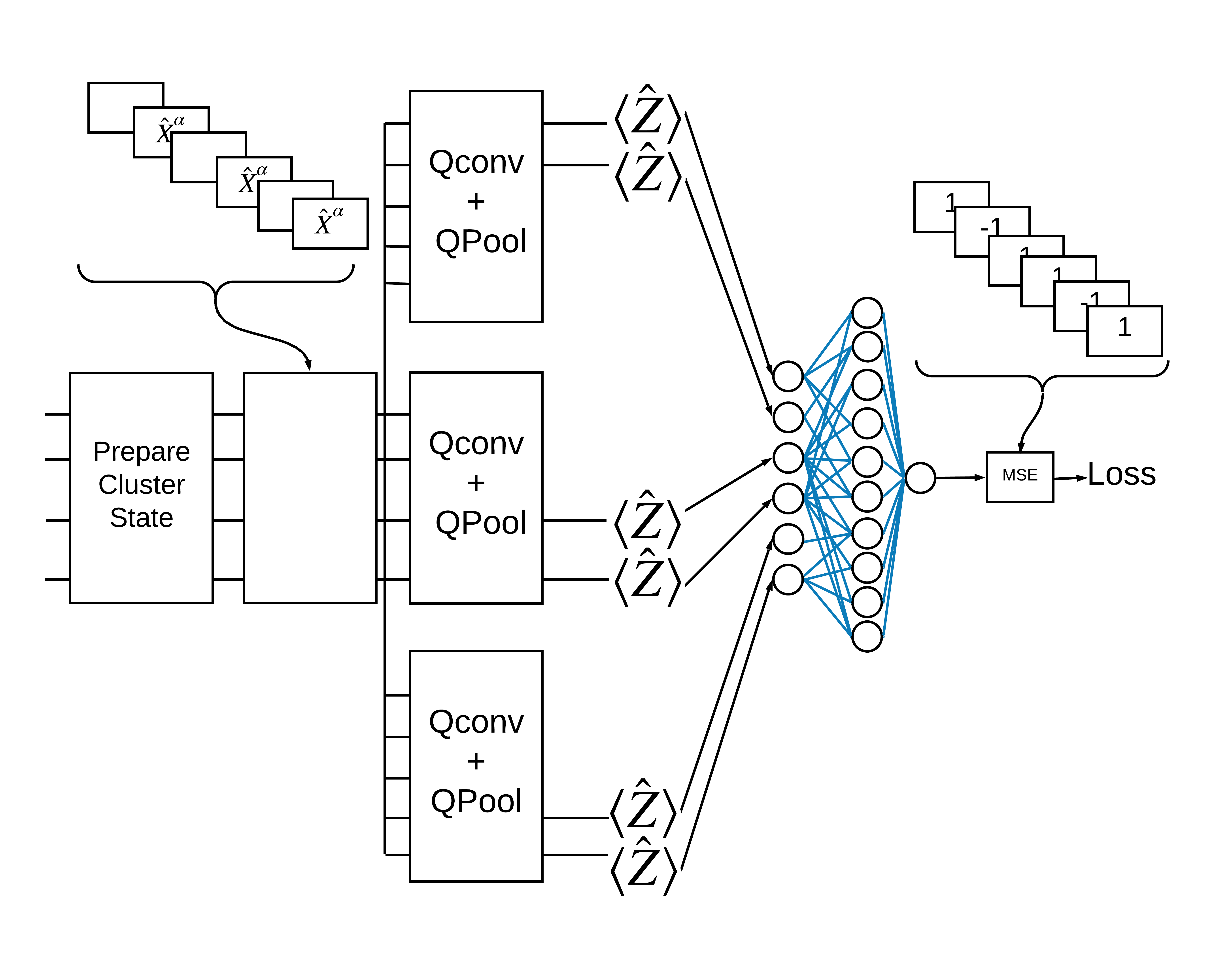
TensorFlow Quantum (TFQ) کلاس های لایه ای را ارائه می دهد که برای ساخت مدار درون گراف طراحی شده اند. یک مثال لایه tfq.layers.AddCircuit است که از tf.keras.Layer به ارث می رسد. همانطور که در شکل زیر نشان داده شده است، این لایه می تواند به دسته مدارهای ورودی اضافه یا اضافه شود.
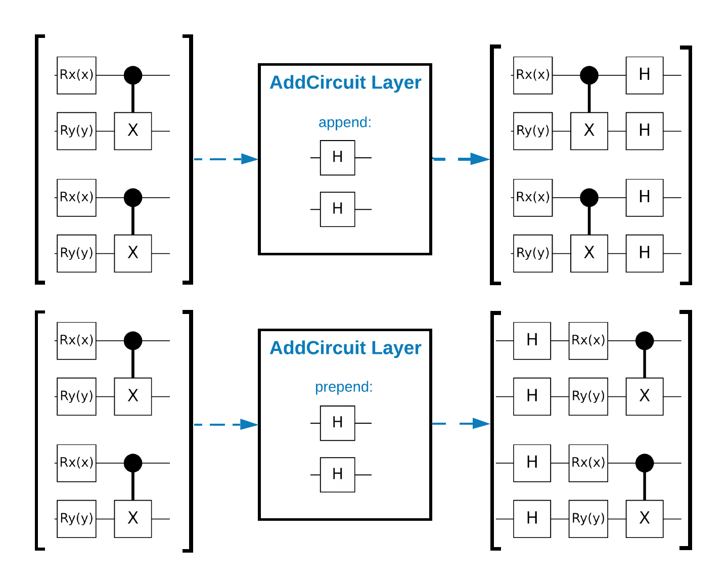
قطعه زیر از این لایه استفاده می کند:
qubit = cirq.GridQubit(0, 0)

# Define some circuits.
circuit1 = cirq.Circuit(cirq.X(qubit))
circuit2 = cirq.Circuit(cirq.H(qubit))

# Convert to a tensor.
input_circuit_tensor = tfq.convert_to_tensor([circuit1, circuit2])

# Define a circuit that we want to append
y_circuit = cirq.Circuit(cirq.Y(qubit))

# Instantiate our layer
y_appender = tfq.layers.AddCircuit()

# Run our circuit tensor through the layer and save the output.
output_circuit_tensor = y_appender(input_circuit_tensor, append=y_circuit)
تانسور ورودی را بررسی کنید:
print(tfq.from_tensor(input_circuit_tensor))
[cirq.Circuit([
     cirq.Moment(
         cirq.X(cirq.GridQubit(0, 0)),
     ),
 ])
 cirq.Circuit([
     cirq.Moment(
         cirq.H(cirq.GridQubit(0, 0)),
     ),
 ])                                   ]
و تانسور خروجی را بررسی کنید:
print(tfq.from_tensor(output_circuit_tensor))
[cirq.Circuit([
     cirq.Moment(
         cirq.X(cirq.GridQubit(0, 0)),
     ),
     cirq.Moment(
         cirq.Y(cirq.GridQubit(0, 0)),
     ),
 ])
 cirq.Circuit([
     cirq.Moment(
         cirq.H(cirq.GridQubit(0, 0)),
     ),
     cirq.Moment(
         cirq.Y(cirq.GridQubit(0, 0)),
     ),
 ])                                   ]
در حالی که میتوان نمونههای زیر را بدون استفاده از tfq.layers.AddCircuit ، اما این فرصت خوبی است برای درک اینکه چگونه عملکردهای پیچیده را میتوان در نمودارهای محاسباتی TensorFlow تعبیه کرد.
1.2 بررسی اجمالی مشکل
شما یک حالت خوشه ای آماده می کنید و یک طبقه بندی کننده کوانتومی را آموزش می دهید تا تشخیص دهد که آیا "هیجان زده" است یا نه. حالت خوشه به شدت درهم تنیده است اما برای یک کامپیوتر کلاسیک لزوما دشوار نیست. برای وضوح، این مجموعه داده ساده تری نسبت به داده مورد استفاده در مقاله است.
برای این کار طبقه بندی، یک معماری عمیق شبیه به MERA QCNN را اجرا خواهید کرد زیرا:
- مانند QCNN، حالت خوشه در یک حلقه از نظر ترجمه ثابت است.
- حالت خوشه ای به شدت درهم تنیده است.
این معماری باید در کاهش درهم تنیدگی، به دست آوردن طبقه بندی با خواندن یک کیوبیت موثر باشد.
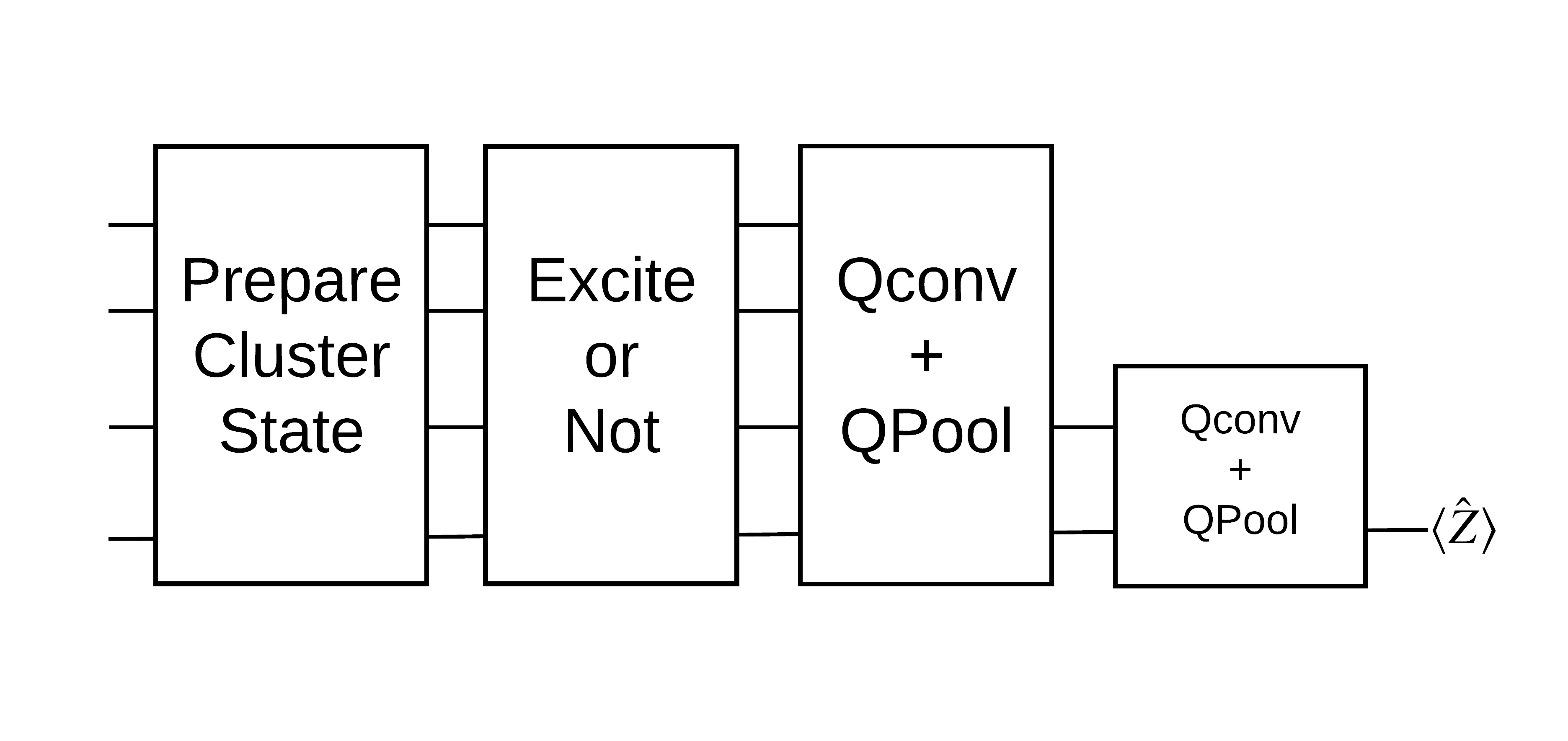
حالت خوشه "تحریک" به عنوان حالت خوشه ای تعریف می شود که دارای یک دروازه cirq.rx برای هر یک از کیوبیت های آن اعمال می شود. Qconv و QPool بعداً در این آموزش مورد بحث قرار می گیرند.
1.3 بلوک های ساختمانی برای TensorFlow
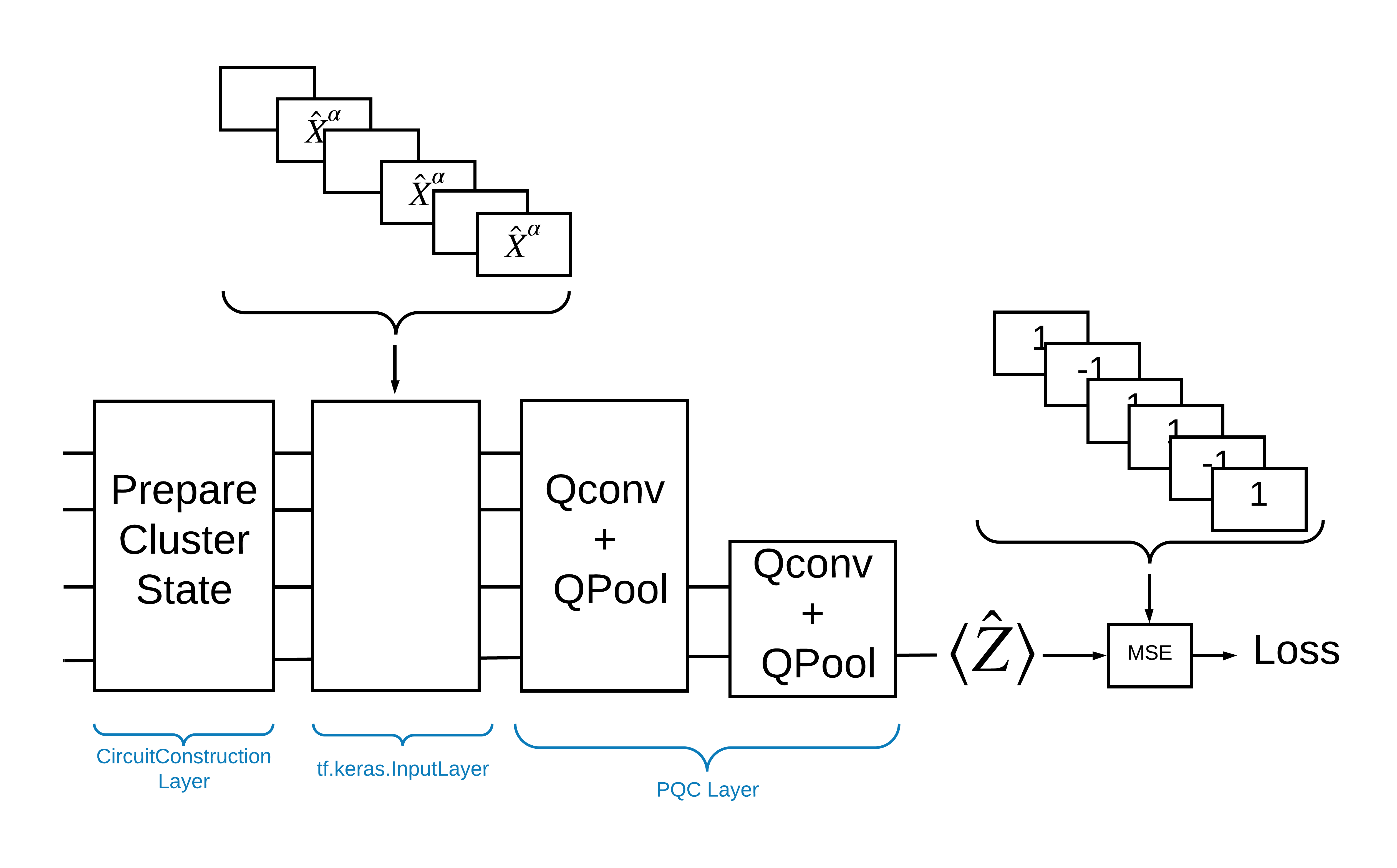
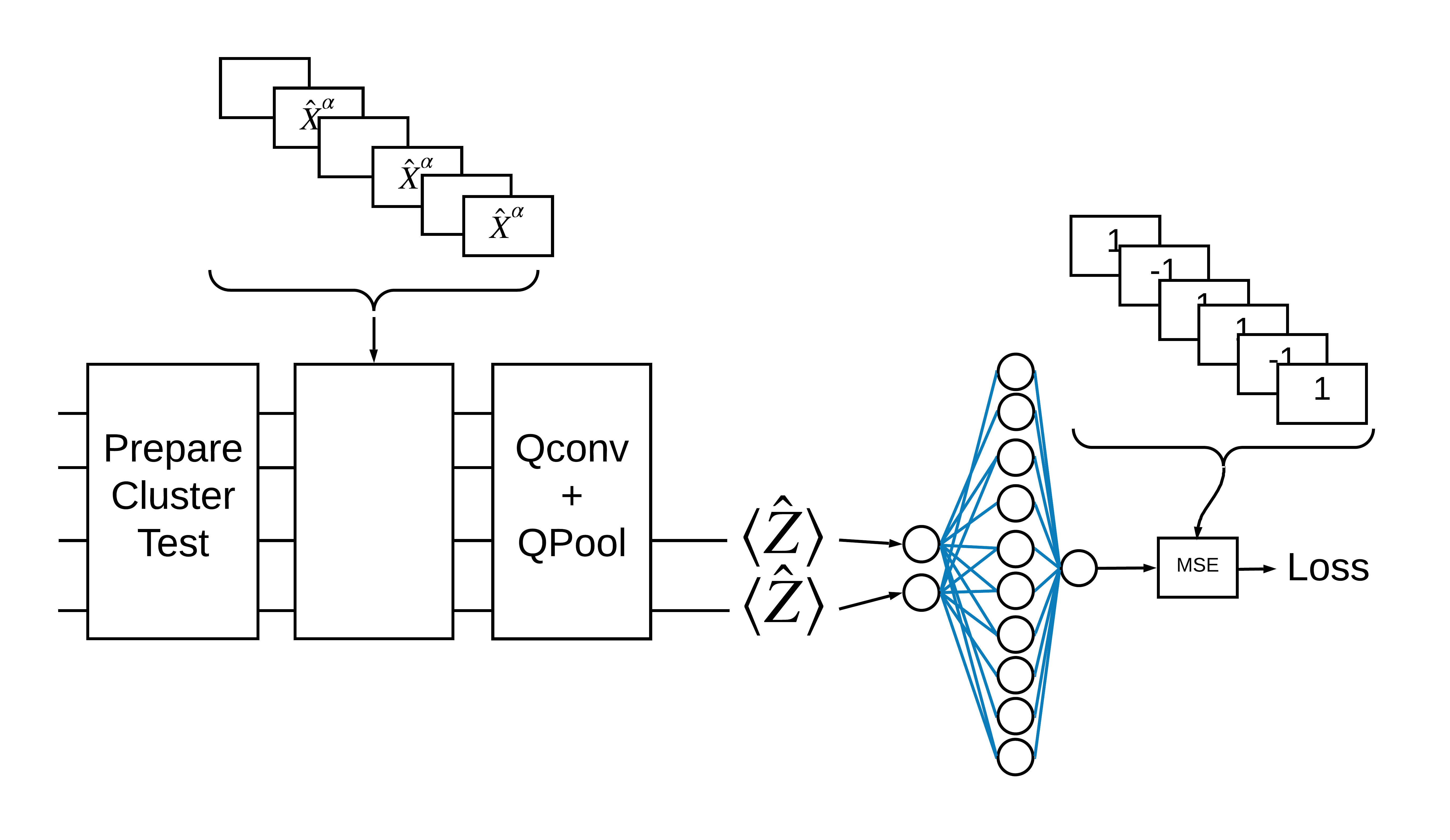
یکی از راههای حل این مشکل با TensorFlow Quantum پیادهسازی موارد زیر است:
- ورودی مدل یک تانسور مدار است - یا یک مدار خالی یا یک گیت X روی یک کیوبیت خاص که نشان دهنده یک تحریک است.
- بقیه اجزای کوانتومی مدل با لایههای
tfq.layers.AddCircuitساخته شدهاند. - برای استنباط از یک لایه
tfq.layers.PQCاستفاده شده است. این \(\langle \hat{Z} \rangle\) را می خواند و آن را با برچسب 1 برای حالت برانگیخته یا -1 برای حالت غیر هیجان زده مقایسه می کند.
1.4 داده ها
قبل از ساخت مدل خود، می توانید داده های خود را تولید کنید. در این مورد، تحریکات به حالت خوشه ای خواهد بود (مقاله اصلی از مجموعه داده پیچیده تری استفاده می کند). تحریکات با دروازه cirq.rx نشان داده می شوند. یک چرخش به اندازه کافی بزرگ به عنوان یک تحریک در نظر گرفته می شود و دارای برچسب 1 است و چرخشی که به اندازه کافی بزرگ نیست دارای برچسب -1 است و به عنوان یک تحریک تلقی نمی شود.
def generate_data(qubits):
    """Generate training and testing data."""
    n_rounds = 20  # Produces n_rounds * n_qubits datapoints.
    excitations = []
    labels = []
    for n in range(n_rounds):
        for bit in qubits:
            rng = np.random.uniform(-np.pi, np.pi)
            excitations.append(cirq.Circuit(cirq.rx(rng)(bit)))
            labels.append(1 if (-np.pi / 2) <= rng <= (np.pi / 2) else -1)

    split_ind = int(len(excitations) * 0.7)
    train_excitations = excitations[:split_ind]
    test_excitations = excitations[split_ind:]

    train_labels = labels[:split_ind]
    test_labels = labels[split_ind:]

    return tfq.convert_to_tensor(train_excitations), np.array(train_labels), \
        tfq.convert_to_tensor(test_excitations), np.array(test_labels)
میتوانید ببینید که دقیقاً مانند یادگیری ماشینی معمولی، یک مجموعه آموزشی و آزمایشی ایجاد میکنید تا از آن برای محک زدن مدل استفاده کنید. می توانید به سرعت به برخی از نقاط داده با استفاده از:
sample_points, sample_labels, _, __ = generate_data(cirq.GridQubit.rect(1, 4))
print('Input:', tfq.from_tensor(sample_points)[0], 'Output:', sample_labels[0])
print('Input:', tfq.from_tensor(sample_points)[1], 'Output:', sample_labels[1])
Input: (0, 0): ───X^0.449─── Output: 1
Input: (0, 1): ───X^-0.74─── Output: -1
1.5 تعریف لایه ها
حالا لایه های نشان داده شده در شکل بالا را در TensorFlow تعریف کنید.
1.5.1 حالت خوشه
اولین گام، تعریف حالت خوشه با استفاده از Cirq ، یک چارچوب ارائه شده توسط گوگل برای برنامه نویسی مدارهای کوانتومی است. از آنجایی که این بخش ایستا از مدل است، آن را با استفاده از قابلیت tfq.layers.AddCircuit جاسازی کنید.
def cluster_state_circuit(bits):
    """Return a cluster state on the qubits in `bits`."""
    circuit = cirq.Circuit()
    circuit.append(cirq.H.on_each(bits))
    for this_bit, next_bit in zip(bits, bits[1:] + [bits[0]]):
        circuit.append(cirq.CZ(this_bit, next_bit))
    return circuit
نمایش یک مدار حالت خوشه ای برای یک مستطیل cirq.GridQubit s:
SVGCircuit(cluster_state_circuit(cirq.GridQubit.rect(1, 4)))
findfont: Font family ['Arial'] not found. Falling back to DejaVu Sans.

1.5.2 لایه های QCNN
لایه هایی که مدل را با استفاده از مقاله Cong و Lukin QCNN تشکیل می دهند را تعریف کنید. چند پیش نیاز وجود دارد:
- ماتریس های واحد پارامتری یک و دو کیوبیتی از مقاله Tucci .
- یک عملیات ادغام دو کیوبیتی با پارامتر کلی.
def one_qubit_unitary(bit, symbols):
    """Make a Cirq circuit enacting a rotation of the bloch sphere about the X,
    Y and Z axis, that depends on the values in `symbols`.
    """
    return cirq.Circuit(
        cirq.X(bit)**symbols[0],
        cirq.Y(bit)**symbols[1],
        cirq.Z(bit)**symbols[2])


def two_qubit_unitary(bits, symbols):
    """Make a Cirq circuit that creates an arbitrary two qubit unitary."""
    circuit = cirq.Circuit()
    circuit += one_qubit_unitary(bits[0], symbols[0:3])
    circuit += one_qubit_unitary(bits[1], symbols[3:6])
    circuit += [cirq.ZZ(*bits)**symbols[6]]
    circuit += [cirq.YY(*bits)**symbols[7]]
    circuit += [cirq.XX(*bits)**symbols[8]]
    circuit += one_qubit_unitary(bits[0], symbols[9:12])
    circuit += one_qubit_unitary(bits[1], symbols[12:])
    return circuit


def two_qubit_pool(source_qubit, sink_qubit, symbols):
    """Make a Cirq circuit to do a parameterized 'pooling' operation, which
    attempts to reduce entanglement down from two qubits to just one."""
    pool_circuit = cirq.Circuit()
    sink_basis_selector = one_qubit_unitary(sink_qubit, symbols[0:3])
    source_basis_selector = one_qubit_unitary(source_qubit, symbols[3:6])
    pool_circuit.append(sink_basis_selector)
    pool_circuit.append(source_basis_selector)
    pool_circuit.append(cirq.CNOT(control=source_qubit, target=sink_qubit))
    pool_circuit.append(sink_basis_selector**-1)
    return pool_circuit
برای دیدن آنچه ایجاد کردید، مدار واحد یک کیوبیتی را چاپ کنید:
SVGCircuit(one_qubit_unitary(cirq.GridQubit(0, 0), sympy.symbols('x0:3')))

و مدار واحد دو کیوبیتی:
SVGCircuit(two_qubit_unitary(cirq.GridQubit.rect(1, 2), sympy.symbols('x0:15')))

و مدار ادغام دو کیوبیتی:
SVGCircuit(two_qubit_pool(*cirq.GridQubit.rect(1, 2), sympy.symbols('x0:6')))

1.5.2.1 کانولوشن کوانتومی
همانطور که در مقاله Cong و Lukin ، کانولوشن کوانتومی 1 بعدی را به عنوان استفاده از یک واحد پارامتری دو کیوبیتی برای هر جفت کیوبیت مجاور با یک گام تعریف کنید.
def quantum_conv_circuit(bits, symbols):
    """Quantum Convolution Layer following the above diagram.
    Return a Cirq circuit with the cascade of `two_qubit_unitary` applied
    to all pairs of qubits in `bits` as in the diagram above.
    """
    circuit = cirq.Circuit()
    for first, second in zip(bits[0::2], bits[1::2]):
        circuit += two_qubit_unitary([first, second], symbols)
    for first, second in zip(bits[1::2], bits[2::2] + [bits[0]]):
        circuit += two_qubit_unitary([first, second], symbols)
    return circuit
نمایش مدار (بسیار افقی):
SVGCircuit(
    quantum_conv_circuit(cirq.GridQubit.rect(1, 8), sympy.symbols('x0:15')))

1.5.2.2 ادغام کوانتومی
یک لایه ادغام کوانتومی از \(N\) کیوبیت به \(\frac{N}{2}\) کیوبیت با استفاده از استخر دو کیوبیتی تعریف شده در بالا، ترکیب می شود.
def quantum_pool_circuit(source_bits, sink_bits, symbols):
    """A layer that specifies a quantum pooling operation.
    A Quantum pool tries to learn to pool the relevant information from two
    qubits onto 1.
    """
    circuit = cirq.Circuit()
    for source, sink in zip(source_bits, sink_bits):
        circuit += two_qubit_pool(source, sink, symbols)
    return circuit
مدار جزء ترکیبی را بررسی کنید:
test_bits = cirq.GridQubit.rect(1, 8)

SVGCircuit(
    quantum_pool_circuit(test_bits[:4], test_bits[4:], sympy.symbols('x0:6')))

1.6 تعریف مدل
اکنون از لایه های تعریف شده برای ساخت یک CNN صرفا کوانتومی استفاده کنید. با هشت کیوبیت شروع کنید، یک عدد جمع کنید، سپس \(\langle \hat{Z} \rangle\)اندازه بگیرید.
def create_model_circuit(qubits):
"""Create sequence of alternating convolution and pooling operators
which gradually shrink over time."""
model_circuit = cirq.Circuit()
symbols = sympy.symbols('qconv0:63')
# Cirq uses sympy.Symbols to map learnable variables. TensorFlow Quantum
# scans incoming circuits and replaces these with TensorFlow variables.
model_circuit += quantum_conv_circuit(qubits, symbols[0:15])
model_circuit += quantum_pool_circuit(qubits[:4], qubits[4:],
symbols[15:21])
model_circuit += quantum_conv_circuit(qubits[4:], symbols[21:36])
model_circuit += quantum_pool_circuit(qubits[4:6], qubits[6:],
symbols[36:42])
model_circuit += quantum_conv_circuit(qubits[6:], symbols[42:57])
model_circuit += quantum_pool_circuit([qubits[6]], [qubits[7]],
symbols[57:63])
return model_circuit
# Create our qubits and readout operators in Cirq.
cluster_state_bits = cirq.GridQubit.rect(1, 8)
readout_operators = cirq.Z(cluster_state_bits[-1])
# Build a sequential model enacting the logic in 1.3 of this notebook.
# Here you are making the static cluster state prep as a part of the AddCircuit and the
# "quantum datapoints" are coming in the form of excitation
excitation_input = tf.keras.Input(shape=(), dtype=tf.dtypes.string)
cluster_state = tfq.layers.AddCircuit()(
excitation_input, prepend=cluster_state_circuit(cluster_state_bits))
quantum_model = tfq.layers.PQC(create_model_circuit(cluster_state_bits),
readout_operators)(cluster_state)
qcnn_model = tf.keras.Model(inputs=[excitation_input], outputs=[quantum_model])
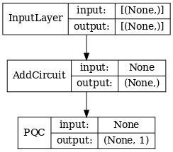
# Show the keras plot of the model
tf.keras.utils.plot_model(qcnn_model,
show_shapes=True,
show_layer_names=False,
dpi=70)
1.7 مدل را آموزش دهید
برای سادهسازی این مثال، مدل را روی دسته کامل آموزش دهید.
# Generate some training data.
train_excitations, train_labels, test_excitations, test_labels = generate_data(
    cluster_state_bits)


# Custom accuracy metric.
@tf.function
def custom_accuracy(y_true, y_pred):
    y_true = tf.squeeze(y_true)
    y_pred = tf.map_fn(lambda x: 1.0 if x >= 0 else -1.0, y_pred)
    return tf.keras.backend.mean(tf.keras.backend.equal(y_true, y_pred))


qcnn_model.compile(optimizer=tf.keras.optimizers.Adam(learning_rate=0.02),
                   loss=tf.losses.mse,
                   metrics=[custom_accuracy])

history = qcnn_model.fit(x=train_excitations,
                         y=train_labels,
                         batch_size=16,
                         epochs=25,
                         verbose=1,
                         validation_data=(test_excitations, test_labels))
Epoch 1/25
7/7 [==============================] - 2s 176ms/step - loss: 0.8961 - custom_accuracy: 0.7143 - val_loss: 0.8012 - val_custom_accuracy: 0.7500
Epoch 2/25
7/7 [==============================] - 1s 140ms/step - loss: 0.7736 - custom_accuracy: 0.7946 - val_loss: 0.7355 - val_custom_accuracy: 0.8542
Epoch 3/25
7/7 [==============================] - 1s 138ms/step - loss: 0.7319 - custom_accuracy: 0.8393 - val_loss: 0.7045 - val_custom_accuracy: 0.8125
Epoch 4/25
7/7 [==============================] - 1s 137ms/step - loss: 0.6976 - custom_accuracy: 0.8482 - val_loss: 0.6829 - val_custom_accuracy: 0.8333
Epoch 5/25
7/7 [==============================] - 1s 143ms/step - loss: 0.6696 - custom_accuracy: 0.8750 - val_loss: 0.6749 - val_custom_accuracy: 0.7917
Epoch 6/25
7/7 [==============================] - 1s 137ms/step - loss: 0.6631 - custom_accuracy: 0.8750 - val_loss: 0.6718 - val_custom_accuracy: 0.7917
Epoch 7/25
7/7 [==============================] - 1s 135ms/step - loss: 0.6536 - custom_accuracy: 0.8929 - val_loss: 0.6638 - val_custom_accuracy: 0.8750
Epoch 8/25
7/7 [==============================] - 1s 141ms/step - loss: 0.6376 - custom_accuracy: 0.8750 - val_loss: 0.6311 - val_custom_accuracy: 0.8542
Epoch 9/25
7/7 [==============================] - 1s 137ms/step - loss: 0.6208 - custom_accuracy: 0.8750 - val_loss: 0.5995 - val_custom_accuracy: 0.8542
Epoch 10/25
7/7 [==============================] - 1s 134ms/step - loss: 0.5887 - custom_accuracy: 0.8661 - val_loss: 0.5655 - val_custom_accuracy: 0.8333
Epoch 11/25
7/7 [==============================] - 1s 144ms/step - loss: 0.5796 - custom_accuracy: 0.8482 - val_loss: 0.5681 - val_custom_accuracy: 0.8333
Epoch 12/25
7/7 [==============================] - 1s 143ms/step - loss: 0.5630 - custom_accuracy: 0.7946 - val_loss: 0.5179 - val_custom_accuracy: 0.8333
Epoch 13/25
7/7 [==============================] - 1s 137ms/step - loss: 0.5405 - custom_accuracy: 0.8304 - val_loss: 0.5003 - val_custom_accuracy: 0.8333
Epoch 14/25
7/7 [==============================] - 1s 138ms/step - loss: 0.5259 - custom_accuracy: 0.8036 - val_loss: 0.4787 - val_custom_accuracy: 0.8333
Epoch 15/25
7/7 [==============================] - 1s 137ms/step - loss: 0.5077 - custom_accuracy: 0.8482 - val_loss: 0.4741 - val_custom_accuracy: 0.8125
Epoch 16/25
7/7 [==============================] - 1s 136ms/step - loss: 0.5082 - custom_accuracy: 0.8214 - val_loss: 0.4739 - val_custom_accuracy: 0.8125
Epoch 17/25
7/7 [==============================] - 1s 137ms/step - loss: 0.5138 - custom_accuracy: 0.8214 - val_loss: 0.4859 - val_custom_accuracy: 0.8750
Epoch 18/25
7/7 [==============================] - 1s 133ms/step - loss: 0.5073 - custom_accuracy: 0.8304 - val_loss: 0.4879 - val_custom_accuracy: 0.8333
Epoch 19/25
7/7 [==============================] - 1s 138ms/step - loss: 0.5084 - custom_accuracy: 0.8304 - val_loss: 0.4745 - val_custom_accuracy: 0.8542
Epoch 20/25
7/7 [==============================] - 1s 139ms/step - loss: 0.5057 - custom_accuracy: 0.8571 - val_loss: 0.4702 - val_custom_accuracy: 0.8333
Epoch 21/25
7/7 [==============================] - 1s 135ms/step - loss: 0.4939 - custom_accuracy: 0.8304 - val_loss: 0.4734 - val_custom_accuracy: 0.8750
Epoch 22/25
7/7 [==============================] - 1s 138ms/step - loss: 0.4942 - custom_accuracy: 0.8750 - val_loss: 0.4725 - val_custom_accuracy: 0.8750
Epoch 23/25
7/7 [==============================] - 1s 140ms/step - loss: 0.4982 - custom_accuracy: 0.9107 - val_loss: 0.4695 - val_custom_accuracy: 0.8958
Epoch 24/25
7/7 [==============================] - 1s 135ms/step - loss: 0.4936 - custom_accuracy: 0.8661 - val_loss: 0.4731 - val_custom_accuracy: 0.8750
Epoch 25/25
7/7 [==============================] - 1s 136ms/step - loss: 0.4866 - custom_accuracy: 0.8571 - val_loss: 0.4631 - val_custom_accuracy: 0.8958
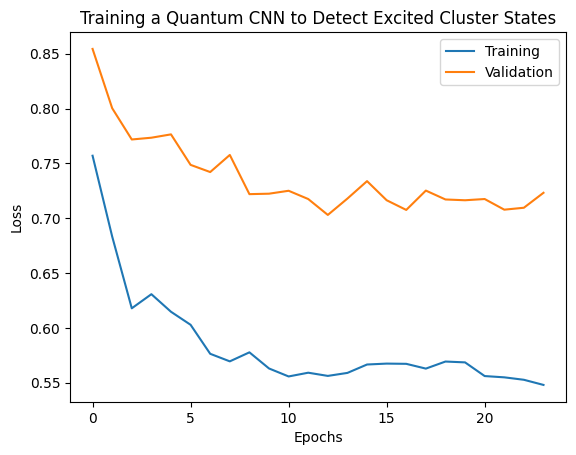
plt.plot(history.history['loss'][1:], label='Training')
plt.plot(history.history['val_loss'][1:], label='Validation')
plt.title('Training a Quantum CNN to Detect Excited Cluster States')
plt.xlabel('Epochs')
plt.ylabel('Loss')
plt.legend()
plt.show()
2. مدل های هیبریدی
شما مجبور نیستید از هشت کیوبیت به یک کیوبیت با استفاده از کانولوشن کوانتومی بروید—شما می توانستید یک یا دو دور کانولوشن کوانتومی انجام دهید و نتایج را به یک شبکه عصبی کلاسیک تغذیه کنید. این بخش به بررسی مدل های ترکیبی کوانتومی-کلاسیک می پردازد.
2.1 مدل هیبریدی با یک فیلتر کوانتومی تک
یک لایه کانولوشن کوانتومی را اعمال کنید، \(\langle \hat{Z}_n \rangle\) را بر روی همه بیت ها بخواند، و به دنبال آن یک شبکه عصبی با اتصال متراکم.
2.1.1 تعریف مدل
# 1-local operators to read out
readouts = [cirq.Z(bit) for bit in cluster_state_bits[4:]]
def multi_readout_model_circuit(qubits):
"""Make a model circuit with less quantum pool and conv operations."""
model_circuit = cirq.Circuit()
symbols = sympy.symbols('qconv0:21')
model_circuit += quantum_conv_circuit(qubits, symbols[0:15])
model_circuit += quantum_pool_circuit(qubits[:4], qubits[4:],
symbols[15:21])
return model_circuit
# Build a model enacting the logic in 2.1 of this notebook.
excitation_input_dual = tf.keras.Input(shape=(), dtype=tf.dtypes.string)
cluster_state_dual = tfq.layers.AddCircuit()(
excitation_input_dual, prepend=cluster_state_circuit(cluster_state_bits))
quantum_model_dual = tfq.layers.PQC(
multi_readout_model_circuit(cluster_state_bits),
readouts)(cluster_state_dual)
d1_dual = tf.keras.layers.Dense(8)(quantum_model_dual)
d2_dual = tf.keras.layers.Dense(1)(d1_dual)
hybrid_model = tf.keras.Model(inputs=[excitation_input_dual], outputs=[d2_dual])
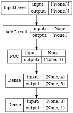
# Display the model architecture
tf.keras.utils.plot_model(hybrid_model,
show_shapes=True,
show_layer_names=False,
dpi=70)
2.1.2 مدل را آموزش دهید
hybrid_model.compile(optimizer=tf.keras.optimizers.Adam(learning_rate=0.02),
                     loss=tf.losses.mse,
                     metrics=[custom_accuracy])

hybrid_history = hybrid_model.fit(x=train_excitations,
                                  y=train_labels,
                                  batch_size=16,
                                  epochs=25,
                                  verbose=1,
                                  validation_data=(test_excitations,
                                                   test_labels))
Epoch 1/25
7/7 [==============================] - 1s 113ms/step - loss: 0.9848 - custom_accuracy: 0.5179 - val_loss: 0.9635 - val_custom_accuracy: 0.5417
Epoch 2/25
7/7 [==============================] - 1s 86ms/step - loss: 0.8095 - custom_accuracy: 0.6339 - val_loss: 0.6800 - val_custom_accuracy: 0.7083
Epoch 3/25
7/7 [==============================] - 1s 85ms/step - loss: 0.4045 - custom_accuracy: 0.9375 - val_loss: 0.3342 - val_custom_accuracy: 0.8750
Epoch 4/25
7/7 [==============================] - 1s 86ms/step - loss: 0.2308 - custom_accuracy: 0.9643 - val_loss: 0.2027 - val_custom_accuracy: 0.9792
Epoch 5/25
7/7 [==============================] - 1s 84ms/step - loss: 0.2232 - custom_accuracy: 0.9554 - val_loss: 0.1761 - val_custom_accuracy: 1.0000
Epoch 6/25
7/7 [==============================] - 1s 84ms/step - loss: 0.1760 - custom_accuracy: 0.9821 - val_loss: 0.2541 - val_custom_accuracy: 0.9167
Epoch 7/25
7/7 [==============================] - 1s 85ms/step - loss: 0.1919 - custom_accuracy: 0.9643 - val_loss: 0.1967 - val_custom_accuracy: 0.9792
Epoch 8/25
7/7 [==============================] - 1s 83ms/step - loss: 0.1892 - custom_accuracy: 0.9554 - val_loss: 0.1870 - val_custom_accuracy: 0.9792
Epoch 9/25
7/7 [==============================] - 1s 84ms/step - loss: 0.1777 - custom_accuracy: 0.9911 - val_loss: 0.2208 - val_custom_accuracy: 0.9583
Epoch 10/25
7/7 [==============================] - 1s 83ms/step - loss: 0.1728 - custom_accuracy: 0.9732 - val_loss: 0.2147 - val_custom_accuracy: 0.9583
Epoch 11/25
7/7 [==============================] - 1s 85ms/step - loss: 0.1704 - custom_accuracy: 0.9732 - val_loss: 0.1810 - val_custom_accuracy: 0.9792
Epoch 12/25
7/7 [==============================] - 1s 85ms/step - loss: 0.1739 - custom_accuracy: 0.9732 - val_loss: 0.2038 - val_custom_accuracy: 0.9792
Epoch 13/25
7/7 [==============================] - 1s 81ms/step - loss: 0.1705 - custom_accuracy: 0.9732 - val_loss: 0.1855 - val_custom_accuracy: 0.9792
Epoch 14/25
7/7 [==============================] - 1s 84ms/step - loss: 0.1788 - custom_accuracy: 0.9643 - val_loss: 0.2152 - val_custom_accuracy: 0.9583
Epoch 15/25
7/7 [==============================] - 1s 84ms/step - loss: 0.1760 - custom_accuracy: 0.9732 - val_loss: 0.1994 - val_custom_accuracy: 1.0000
Epoch 16/25
7/7 [==============================] - 1s 83ms/step - loss: 0.1737 - custom_accuracy: 0.9732 - val_loss: 0.2035 - val_custom_accuracy: 0.9792
Epoch 17/25
7/7 [==============================] - 1s 82ms/step - loss: 0.1749 - custom_accuracy: 0.9911 - val_loss: 0.1983 - val_custom_accuracy: 0.9583
Epoch 18/25
7/7 [==============================] - 1s 83ms/step - loss: 0.1875 - custom_accuracy: 0.9732 - val_loss: 0.1916 - val_custom_accuracy: 0.9583
Epoch 19/25
7/7 [==============================] - 1s 82ms/step - loss: 0.1605 - custom_accuracy: 0.9732 - val_loss: 0.1782 - val_custom_accuracy: 0.9792
Epoch 20/25
7/7 [==============================] - 1s 84ms/step - loss: 0.1668 - custom_accuracy: 0.9911 - val_loss: 0.2276 - val_custom_accuracy: 0.9583
Epoch 21/25
7/7 [==============================] - 1s 84ms/step - loss: 0.1700 - custom_accuracy: 0.9911 - val_loss: 0.2080 - val_custom_accuracy: 0.9583
Epoch 22/25
7/7 [==============================] - 1s 83ms/step - loss: 0.1621 - custom_accuracy: 0.9732 - val_loss: 0.1851 - val_custom_accuracy: 0.9375
Epoch 23/25
7/7 [==============================] - 1s 84ms/step - loss: 0.1695 - custom_accuracy: 0.9911 - val_loss: 0.1882 - val_custom_accuracy: 0.9792
Epoch 24/25
7/7 [==============================] - 1s 82ms/step - loss: 0.1583 - custom_accuracy: 0.9911 - val_loss: 0.2017 - val_custom_accuracy: 0.9583
Epoch 25/25
7/7 [==============================] - 1s 83ms/step - loss: 0.1557 - custom_accuracy: 0.9911 - val_loss: 0.1907 - val_custom_accuracy: 0.9792
plt.plot(history.history['val_custom_accuracy'], label='QCNN')
plt.plot(hybrid_history.history['val_custom_accuracy'], label='Hybrid CNN')
plt.title('Quantum vs Hybrid CNN performance')
plt.xlabel('Epochs')
plt.legend()
plt.ylabel('Validation Accuracy')
plt.show()
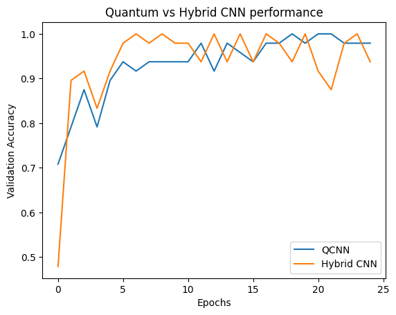
همانطور که می بینید، با کمک کلاسیک بسیار متوسط، مدل هیبریدی معمولاً سریعتر از نسخه کوانتومی خالص همگرا می شود.
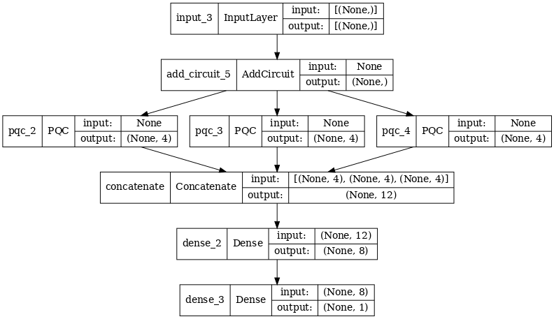
2.2 پیچیدگی هیبریدی با فیلترهای کوانتومی متعدد
اکنون بیایید معماری را امتحان کنیم که از کانولوشن های کوانتومی متعدد و یک شبکه عصبی کلاسیک برای ترکیب آنها استفاده می کند.
2.2.1 تعریف مدل
excitation_input_multi = tf.keras.Input(shape=(), dtype=tf.dtypes.string)

cluster_state_multi = tfq.layers.AddCircuit()(
    excitation_input_multi, prepend=cluster_state_circuit(cluster_state_bits))

# apply 3 different filters and measure expectation values

quantum_model_multi1 = tfq.layers.PQC(
    multi_readout_model_circuit(cluster_state_bits),
    readouts)(cluster_state_multi)

quantum_model_multi2 = tfq.layers.PQC(
    multi_readout_model_circuit(cluster_state_bits),
    readouts)(cluster_state_multi)

quantum_model_multi3 = tfq.layers.PQC(
    multi_readout_model_circuit(cluster_state_bits),
    readouts)(cluster_state_multi)

# concatenate outputs and feed into a small classical NN
concat_out = tf.keras.layers.concatenate(
    [quantum_model_multi1, quantum_model_multi2, quantum_model_multi3])

dense_1 = tf.keras.layers.Dense(8)(concat_out)

dense_2 = tf.keras.layers.Dense(1)(dense_1)

multi_qconv_model = tf.keras.Model(inputs=[excitation_input_multi],
                                   outputs=[dense_2])

# Display the model architecture
tf.keras.utils.plot_model(multi_qconv_model,
                          show_shapes=True,
                          show_layer_names=True,
                          dpi=70)
2.2.2 مدل را آموزش دهید
multi_qconv_model.compile(
    optimizer=tf.keras.optimizers.Adam(learning_rate=0.02),
    loss=tf.losses.mse,
    metrics=[custom_accuracy])

multi_qconv_history = multi_qconv_model.fit(x=train_excitations,
                                            y=train_labels,
                                            batch_size=16,
                                            epochs=25,
                                            verbose=1,
                                            validation_data=(test_excitations,
                                                             test_labels))
Epoch 1/25
7/7 [==============================] - 2s 143ms/step - loss: 0.9425 - custom_accuracy: 0.6429 - val_loss: 0.8120 - val_custom_accuracy: 0.7083
Epoch 2/25
7/7 [==============================] - 1s 109ms/step - loss: 0.5778 - custom_accuracy: 0.7946 - val_loss: 0.5920 - val_custom_accuracy: 0.7500
Epoch 3/25
7/7 [==============================] - 1s 103ms/step - loss: 0.4954 - custom_accuracy: 0.9018 - val_loss: 0.4568 - val_custom_accuracy: 0.7708
Epoch 4/25
7/7 [==============================] - 1s 95ms/step - loss: 0.2855 - custom_accuracy: 0.9196 - val_loss: 0.2792 - val_custom_accuracy: 0.9375
Epoch 5/25
7/7 [==============================] - 1s 93ms/step - loss: 0.1902 - custom_accuracy: 0.9821 - val_loss: 0.2212 - val_custom_accuracy: 0.9375
Epoch 6/25
7/7 [==============================] - 1s 94ms/step - loss: 0.1685 - custom_accuracy: 0.9821 - val_loss: 0.2341 - val_custom_accuracy: 0.9583
Epoch 7/25
7/7 [==============================] - 1s 104ms/step - loss: 0.1671 - custom_accuracy: 0.9911 - val_loss: 0.2062 - val_custom_accuracy: 0.9792
Epoch 8/25
7/7 [==============================] - 1s 97ms/step - loss: 0.1511 - custom_accuracy: 0.9821 - val_loss: 0.2096 - val_custom_accuracy: 0.9792
Epoch 9/25
7/7 [==============================] - 1s 96ms/step - loss: 0.1432 - custom_accuracy: 0.9911 - val_loss: 0.2330 - val_custom_accuracy: 0.9375
Epoch 10/25
7/7 [==============================] - 1s 92ms/step - loss: 0.1668 - custom_accuracy: 0.9821 - val_loss: 0.2344 - val_custom_accuracy: 0.9583
Epoch 11/25
7/7 [==============================] - 1s 106ms/step - loss: 0.1893 - custom_accuracy: 0.9732 - val_loss: 0.2148 - val_custom_accuracy: 0.9583
Epoch 12/25
7/7 [==============================] - 1s 104ms/step - loss: 0.1857 - custom_accuracy: 0.9732 - val_loss: 0.2739 - val_custom_accuracy: 0.9583
Epoch 13/25
7/7 [==============================] - 1s 106ms/step - loss: 0.1748 - custom_accuracy: 0.9732 - val_loss: 0.2366 - val_custom_accuracy: 0.9583
Epoch 14/25
7/7 [==============================] - 1s 103ms/step - loss: 0.1515 - custom_accuracy: 0.9821 - val_loss: 0.2012 - val_custom_accuracy: 0.9583
Epoch 15/25
7/7 [==============================] - 1s 100ms/step - loss: 0.1552 - custom_accuracy: 0.9911 - val_loss: 0.2404 - val_custom_accuracy: 0.9375
Epoch 16/25
7/7 [==============================] - 1s 97ms/step - loss: 0.1572 - custom_accuracy: 0.9911 - val_loss: 0.2779 - val_custom_accuracy: 0.9375
Epoch 17/25
7/7 [==============================] - 1s 100ms/step - loss: 0.1546 - custom_accuracy: 0.9821 - val_loss: 0.2104 - val_custom_accuracy: 0.9583
Epoch 18/25
7/7 [==============================] - 1s 102ms/step - loss: 0.1418 - custom_accuracy: 0.9911 - val_loss: 0.2647 - val_custom_accuracy: 0.9583
Epoch 19/25
7/7 [==============================] - 1s 98ms/step - loss: 0.1590 - custom_accuracy: 0.9732 - val_loss: 0.2154 - val_custom_accuracy: 0.9583
Epoch 20/25
7/7 [==============================] - 1s 104ms/step - loss: 0.1363 - custom_accuracy: 1.0000 - val_loss: 0.2470 - val_custom_accuracy: 0.9375
Epoch 21/25
7/7 [==============================] - 1s 100ms/step - loss: 0.1442 - custom_accuracy: 0.9821 - val_loss: 0.2383 - val_custom_accuracy: 0.9375
Epoch 22/25
7/7 [==============================] - 1s 99ms/step - loss: 0.1415 - custom_accuracy: 0.9911 - val_loss: 0.2324 - val_custom_accuracy: 0.9583
Epoch 23/25
7/7 [==============================] - 1s 97ms/step - loss: 0.1424 - custom_accuracy: 0.9821 - val_loss: 0.2188 - val_custom_accuracy: 0.9583
Epoch 24/25
7/7 [==============================] - 1s 100ms/step - loss: 0.1417 - custom_accuracy: 0.9821 - val_loss: 0.2340 - val_custom_accuracy: 0.9375
Epoch 25/25
7/7 [==============================] - 1s 103ms/step - loss: 0.1471 - custom_accuracy: 0.9732 - val_loss: 0.2252 - val_custom_accuracy: 0.9583
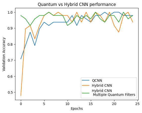
plt.plot(history.history['val_custom_accuracy'][:25], label='QCNN')
plt.plot(hybrid_history.history['val_custom_accuracy'][:25], label='Hybrid CNN')
plt.plot(multi_qconv_history.history['val_custom_accuracy'][:25],
         label='Hybrid CNN \n Multiple Quantum Filters')
plt.title('Quantum vs Hybrid CNN performance')
plt.xlabel('Epochs')
plt.legend()
plt.ylabel('Validation Accuracy')
plt.show()