
|
|
|
 View source on GitHub View source on GitHub
|
|
Overview
DTensor provides a way for you to distribute the training of your model across devices to improve efficiency, reliability and scalability. For more details, check out the DTensor concepts guide.
In this tutorial, you will train a sentiment analysis model using DTensors. The example demonstrates three distributed training schemes:
- Data Parallel training, where the training samples are sharded (partitioned) to devices.
- Model Parallel training, where the model variables are sharded to devices.
- Spatial Parallel training, where the features of input data are sharded to devices (also known as Spatial Partitioning).
The training portion of this tutorial is inspired by a Kaggle notebook called A Kaggle guide on sentiment analysis. To learn about the complete training and evaluation workflow (without DTensor), refer to that notebook.
This tutorial will walk through the following steps:
- Some data cleaning to obtain a
tf.data.Datasetof tokenized sentences and their polarity. - Then, building an MLP model with custom Dense and BatchNorm layers using a
tf.Moduleto track the inference variables. The model constructor will take additionalLayoutarguments to control the sharding of variables. - For training, you will first use data parallel training together with
tf.experimental.dtensor's checkpoint feature. Then, you will continue with Model Parallel Training and Spatial Parallel Training. - The final section briefly describes the interaction between
tf.saved_modelandtf.experimental.dtensoras of TensorFlow 2.9.
Setup
DTensor (tf.experimental.dtensor) has been part of TensorFlow since the 2.9.0 release.
First, install or upgrade TensorFlow Datasets:
pip install --quiet --upgrade tensorflow-datasetsNext, import tensorflow and dtensor, and configure TensorFlow to use 8 virtual CPUs.
Even though this example uses virtual CPUs, DTensor works the same way on CPU, GPU or TPU devices.
import tempfile
import numpy as np
import tensorflow_datasets as tfds

import tensorflow as tf

from tensorflow.experimental import dtensor

print('TensorFlow version:', tf.__version__)
def configure_virtual_cpus(ncpu):
  phy_devices = tf.config.list_physical_devices('CPU')
  tf.config.set_logical_device_configuration(phy_devices[0], [
        tf.config.LogicalDeviceConfiguration(),
    ] * ncpu)

configure_virtual_cpus(8)
DEVICES = [f'CPU:{i}' for i in range(8)]

tf.config.list_logical_devices('CPU')
Download the dataset
Download the IMDB reviews data set to train the sentiment analysis model:
train_data = tfds.load('imdb_reviews', split='train', shuffle_files=True, batch_size=64)
train_data
Prepare the data
First tokenize the text. Here use an extension of one-hot encoding, the 'tf_idf' mode of tf.keras.layers.TextVectorization.
- For the sake of speed, limit the number of tokens to 1200.
- To keep the
tf.Modulesimple, runTextVectorizationas a preprocessing step before the training.
The final result of the data cleaning section is a Dataset with the tokenized text as x and label as y.
text_vectorization = tf.keras.layers.TextVectorization(output_mode='tf_idf', max_tokens=1200, output_sequence_length=None)
text_vectorization.adapt(data=train_data.map(lambda x: x['text']))
def vectorize(features):
  return text_vectorization(features['text']), features['label']

train_data_vec = train_data.map(vectorize)
train_data_vec
Build a neural network with DTensor
Now build a Multi-Layer Perceptron (MLP) network with DTensor. The network will use fully connected Dense and BatchNorm layers.
DTensor expands TensorFlow through single-program multi-data (SPMD) expansion of regular TensorFlow Ops according to the dtensor.Layout attributes of their input Tensor and variables.
Variables of DTensor aware layers are dtensor.DVariable, and the constructors of DTensor aware layer objects take additional Layout inputs in addition to the usual layer parameters.
Dense Layer
The following custom Dense layer defines 2 layer variables: \(W_{ij}\) is the variable for weights, and \(b_i\) is the variable for the biases.
\[ y_j = \sigma(\sum_i x_i W_{ij} + b_j) \]
Layout deduction
This result comes from the following observations:
The preferred DTensor sharding for operands to a matrix dot product \(t_j = \sum_i x_i W_{ij}\) is to shard \(\mathbf{W}\) and \(\mathbf{x}\) the same way along the \(i\)-axis.
The preferred DTensor sharding for operands to a matrix sum \(t_j + b_j\), is to shard \(\mathbf{t}\) and \(\mathbf{b}\) the same way along the \(j\)-axis.
class Dense(tf.Module):

  def __init__(self, input_size, output_size,
               init_seed, weight_layout, activation=None):
    super().__init__()

    random_normal_initializer = tf.function(tf.random.stateless_normal)

    self.weight = dtensor.DVariable(
        dtensor.call_with_layout(
            random_normal_initializer, weight_layout,
            shape=[input_size, output_size],
            seed=init_seed
            ))
    if activation is None:
      activation = lambda x:x
    self.activation = activation

    # bias is sharded the same way as the last axis of weight.
    bias_layout = weight_layout.delete([0])

    self.bias = dtensor.DVariable(
        dtensor.call_with_layout(tf.zeros, bias_layout, [output_size]))

  def __call__(self, x):
    y = tf.matmul(x, self.weight) + self.bias
    y = self.activation(y)

    return y
BatchNorm
A batch normalization layer helps avoid collapsing modes while training. In this case, adding batch normalization layers helps model training avoid producing a model that only produces zeros.
The constructor of the custom BatchNorm layer below does not take a Layout argument. This is because BatchNorm has no layer variables. This still works with DTensor because 'x', the only input to the layer, is already a DTensor that represents the global batch.
class BatchNorm(tf.Module):

  def __init__(self):
    super().__init__()

  def __call__(self, x, training=True):
    if not training:
      # This branch is not used in the Tutorial.
      pass
    mean, variance = tf.nn.moments(x, axes=[0])
    return tf.nn.batch_normalization(x, mean, variance, 0.0, 1.0, 1e-5)
A full featured batch normalization layer (such as tf.keras.layers.BatchNormalization) will need Layout arguments for its variables.
def make_keras_bn(bn_layout):
  return tf.keras.layers.BatchNormalization(gamma_layout=bn_layout,
                                            beta_layout=bn_layout,
                                            moving_mean_layout=bn_layout,
                                            moving_variance_layout=bn_layout,
                                            fused=False)
Putting Layers Together
Next, build a Multi-layer perceptron (MLP) network with the building blocks above. The diagram below shows the axis relationships between the input x and the weight matrices for the two Dense layers without any DTensor sharding or replication applied.
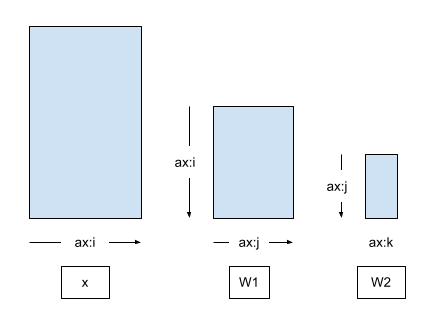
The output of the first Dense layer is passed into the input of the second Dense layer (after the BatchNorm). Therefore, the preferred DTensor sharding for the output of first Dense layer (\(\mathbf{W_1}\)) and the input of second Dense layer (\(\mathbf{W_2}\)) is to shard \(\mathbf{W_1}\) and \(\mathbf{W_2}\) the same way along the common axis \(\hat{j}\),
\[ \mathsf{Layout}[{W_{1,ij} }; i, j] = \left[\hat{i}, \hat{j}\right] \\ \mathsf{Layout}[{W_{2,jk} }; j, k] = \left[\hat{j}, \hat{k} \right] \]
Even though the layout deduction shows that the 2 layouts are not independent, for the sake of simplicity of the model interface, MLP will take 2 Layout arguments, one per Dense layer.
from typing import Tuple

class MLP(tf.Module):

  def __init__(self, dense_layouts: Tuple[dtensor.Layout, dtensor.Layout]):
    super().__init__()

    self.dense1 = Dense(
        1200, 48, (1, 2), dense_layouts[0], activation=tf.nn.relu)
    self.bn = BatchNorm()
    self.dense2 = Dense(48, 2, (3, 4), dense_layouts[1])

  def __call__(self, x):
    y = x
    y = self.dense1(y)
    y = self.bn(y)
    y = self.dense2(y)
    return y
The trade-off between correctness in layout deduction constraints and simplicity of API is a common design point of APIs that uses DTensor.
It is also possible to capture the dependency between Layout's with a different API. For example, the MLPStricter class creates the Layout objects in the constructor.
class MLPStricter(tf.Module):

  def __init__(self, mesh, input_mesh_dim, inner_mesh_dim1, output_mesh_dim):
    super().__init__()

    self.dense1 = Dense(
        1200, 48, (1, 2), dtensor.Layout([input_mesh_dim, inner_mesh_dim1], mesh),
        activation=tf.nn.relu)
    self.bn = BatchNorm()
    self.dense2 = Dense(48, 2, (3, 4), dtensor.Layout([inner_mesh_dim1, output_mesh_dim], mesh))


  def __call__(self, x):
    y = x
    y = self.dense1(y)
    y = self.bn(y)
    y = self.dense2(y)
    return y
To make sure the model runs, probe your model with fully replicated layouts and a fully replicated batch of 'x' input.
WORLD = dtensor.create_mesh([("world", 8)], devices=DEVICES)

model = MLP([dtensor.Layout.replicated(WORLD, rank=2),
             dtensor.Layout.replicated(WORLD, rank=2)])

sample_x, sample_y = train_data_vec.take(1).get_single_element()
sample_x = dtensor.copy_to_mesh(sample_x, dtensor.Layout.replicated(WORLD, rank=2))
print(model(sample_x))
Moving data to the device
Usually, tf.data iterators (and other data fetching methods) yield tensor objects backed by the local host device memory. This data must be transferred to the accelerator device memory that backs DTensor's component tensors.
dtensor.copy_to_mesh is unsuitable for this situation because it replicates input tensors to all devices due to DTensor's global perspective. So in this tutorial, you will use a helper function repack_local_tensor, to facilitate the transfer of data. This helper function uses dtensor.pack to send (and only send) the shard of the global batch that is intended for a replica to the device backing the replica.
This simplified function assumes single-client. Determining the correct way to split the local tensor and the mapping between the pieces of the split and the local devices can be laboring in a multi-client application.
Additional DTensor API to simplify tf.data integration is planned, supporting both single-client and multi-client applications. Please stay tuned.
def repack_local_tensor(x, layout):
  """Repacks a local Tensor-like to a DTensor with layout.

  This function assumes a single-client application.
  """
  x = tf.convert_to_tensor(x)
  sharded_dims = []

  # For every sharded dimension, use tf.split to split the along the dimension.
  # The result is a nested list of split-tensors in queue[0].
  queue = [x]
  for axis, dim in enumerate(layout.sharding_specs):
    if dim == dtensor.UNSHARDED:
      continue
    num_splits = layout.shape[axis]
    queue = tf.nest.map_structure(lambda x: tf.split(x, num_splits, axis=axis), queue)
    sharded_dims.append(dim)

  # Now we can build the list of component tensors by looking up the location in
  # the nested list of split-tensors created in queue[0].
  components = []
  for locations in layout.mesh.local_device_locations():
    t = queue[0]
    for dim in sharded_dims:
      split_index = locations[dim]  # Only valid on single-client mesh.
      t = t[split_index]
    components.append(t)

  return dtensor.pack(components, layout)
Data parallel training
In this section, you will train your MLP model with data parallel training. The following sections will demonstrate model parallel training and spatial parallel training.
Data parallel training is a commonly used scheme for distributed machine learning:
- Model variables are replicated on N devices each.
- A global batch is split into N per-replica batches.
- Each per-replica batch is trained on the replica device.
- The gradient is reduced before weight up data is collectively performed on all replicas.
Data parallel training provides nearly linear speedup regarding the number of devices.
Creating a data parallel mesh
A typical data parallelism training loop uses a DTensor Mesh that consists of a single batch dimension, where each device becomes a replica that receives a shard from the global batch.
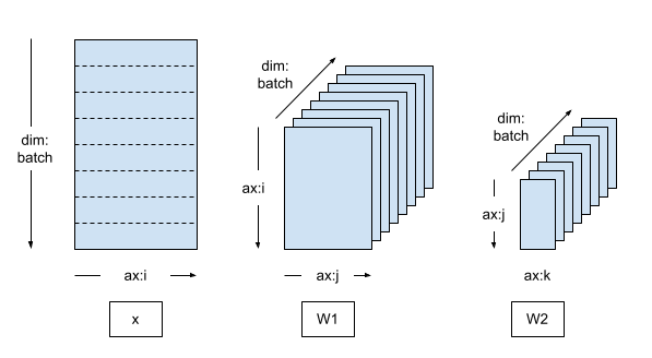
The replicated model runs on the replica, therefore the model variables are fully replicated (unsharded).
mesh = dtensor.create_mesh([("batch", 8)], devices=DEVICES)

model = MLP([dtensor.Layout([dtensor.UNSHARDED, dtensor.UNSHARDED], mesh),
             dtensor.Layout([dtensor.UNSHARDED, dtensor.UNSHARDED], mesh),])
Packing training data to DTensors
The training data batch should be packed into DTensors sharded along the 'batch'(first) axis, such that DTensor will evenly distribute the training data to the 'batch' mesh dimension.
def repack_batch(x, y, mesh):
  x = repack_local_tensor(x, layout=dtensor.Layout(['batch', dtensor.UNSHARDED], mesh))
  y = repack_local_tensor(y, layout=dtensor.Layout(['batch'], mesh))
  return x, y

sample_x, sample_y = train_data_vec.take(1).get_single_element()
sample_x, sample_y = repack_batch(sample_x, sample_y, mesh)

print('x', sample_x[:, 0])
print('y', sample_y)
Training step
This example uses a Stochastic Gradient Descent optimizer with the Custom Training Loop (CTL). Consult the Custom Training Loop guide and Walk through for more information on those topics.
The train_step is encapsulated as a tf.function to indicate this body is to be traced as a TensorFlow Graph. The body of train_step consists of a forward inference pass, a backward gradient pass, and the variable update.
Note that the body of train_step does not contain any special DTensor annotations. Instead, train_step only contains high-level TensorFlow operations that process the input x and y from the global view of the input batch and the model. All of the DTensor annotations (Mesh, Layout) are factored out of the train step.
# Refer to the CTL (custom training loop guide)
@tf.function
def train_step(model, x, y, learning_rate=tf.constant(1e-4)):
  with tf.GradientTape() as tape:
    logits = model(x)
    # tf.reduce_sum sums the batch sharded per-example loss to a replicated
    # global loss (scalar).
    loss = tf.reduce_sum(
        tf.nn.sparse_softmax_cross_entropy_with_logits(
            logits=logits, labels=y))
  parameters = model.trainable_variables
  gradients = tape.gradient(loss, parameters)
  for parameter, parameter_gradient in zip(parameters, gradients):
    parameter.assign_sub(learning_rate * parameter_gradient)

  # Define some metrics
  accuracy = 1.0 - tf.reduce_sum(tf.cast(tf.argmax(logits, axis=-1, output_type=tf.int64) != y, tf.float32)) / x.shape[0]
  loss_per_sample = loss / len(x)
  return {'loss': loss_per_sample, 'accuracy': accuracy}
Checkpointing
You can checkpoint a DTensor model using tf.train.Checkpoint out of the box. Saving and restoring sharded DVariables will perform an efficient sharded save and restore. Currently, when using tf.train.Checkpoint.save and tf.train.Checkpoint.restore, all DVariables must be on the same host mesh, and DVariables and regular variables cannot be saved together. You can learn more about checkpointing in this guide.
When a DTensor checkpoint is restored, Layouts of variables can be different from when the checkpoint is saved. That is, saving DTensor models is layout- and mesh-agnostic, and only affects the efficiency of sharded saving. You can save a DTensor model with one mesh and layout and restore it on a different mesh and layout. This tutorial makes use of this feature to continue the training in the Model Parallel training and Spatial Parallel training sections.
CHECKPOINT_DIR = tempfile.mkdtemp()

def start_checkpoint_manager(model):
  ckpt = tf.train.Checkpoint(root=model)
  manager = tf.train.CheckpointManager(ckpt, CHECKPOINT_DIR, max_to_keep=3)

  if manager.latest_checkpoint:
    print("Restoring a checkpoint")
    ckpt.restore(manager.latest_checkpoint).assert_consumed()
  else:
    print("New training")
  return manager
Training loop
For the data parallel training scheme, train for epochs and report the progress. 3 epochs is insufficient for training the model -- an accuracy of 50% is as good as randomly guessing.
Enable checkpointing so that you can pick up the training later. In the following section, you will load the checkpoint and train with a different parallel scheme.
num_epochs = 2
manager = start_checkpoint_manager(model)

for epoch in range(num_epochs):
  step = 0
  pbar = tf.keras.utils.Progbar(target=int(train_data_vec.cardinality()), stateful_metrics=[])
  metrics = {'epoch': epoch}
  for x,y in train_data_vec:

    x, y = repack_batch(x, y, mesh)

    metrics.update(train_step(model, x, y, 1e-2))

    pbar.update(step, values=metrics.items(), finalize=False)
    step += 1
  manager.save()
  pbar.update(step, values=metrics.items(), finalize=True)
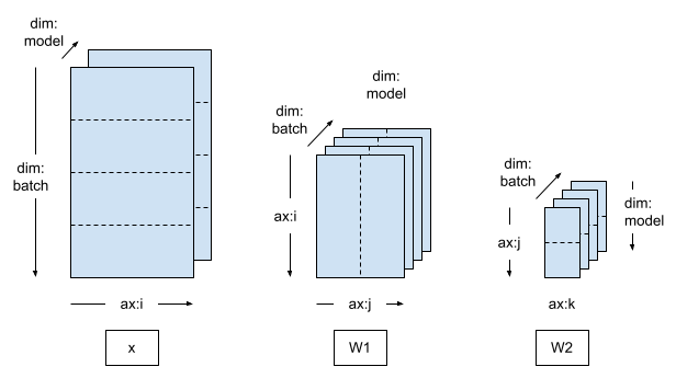
Model Parallel Training
If you switch to a 2 dimensional Mesh, and shard the model variables along the second mesh dimension, then the training becomes Model Parallel.
In Model Parallel training, each model replica spans multiple devices (2 in this case):
- There are 4 model replicas, and the training data batch is distributed to the 4 replicas.
- The 2 devices within a single model replica receive replicated training data.
mesh = dtensor.create_mesh([("batch", 4), ("model", 2)], devices=DEVICES)
model = MLP([dtensor.Layout([dtensor.UNSHARDED, "model"], mesh),
             dtensor.Layout(["model", dtensor.UNSHARDED], mesh)])
As the training data is still sharded along the batch dimension, you can reuse the same repack_batch function as the Data Parallel training case. DTensor will automatically replicate the per-replica batch to all devices inside the replica along the "model" mesh dimension.
def repack_batch(x, y, mesh):
  x = repack_local_tensor(x, layout=dtensor.Layout(['batch', dtensor.UNSHARDED], mesh))
  y = repack_local_tensor(y, layout=dtensor.Layout(['batch'], mesh))
  return x, y
Next run the training loop. The training loop reuses the same checkpoint manager as the Data Parallel training example, and the code looks identical.
You can continue training the data parallel trained model under model parallel training.
num_epochs = 2
manager = start_checkpoint_manager(model)

for epoch in range(num_epochs):
  step = 0
  pbar = tf.keras.utils.Progbar(target=int(train_data_vec.cardinality()))
  metrics = {'epoch': epoch}
  for x,y in train_data_vec:
    x, y = repack_batch(x, y, mesh)
    metrics.update(train_step(model, x, y, 1e-2))
    pbar.update(step, values=metrics.items(), finalize=False)
    step += 1
  manager.save()
  pbar.update(step, values=metrics.items(), finalize=True)
Spatial Parallel Training
When training data of very high dimensionality (e.g. a very large image or a video), it may be desirable to shard along the feature dimension. This is called Spatial Partitioning, which was first introduced into TensorFlow for training models with large 3-d input samples.
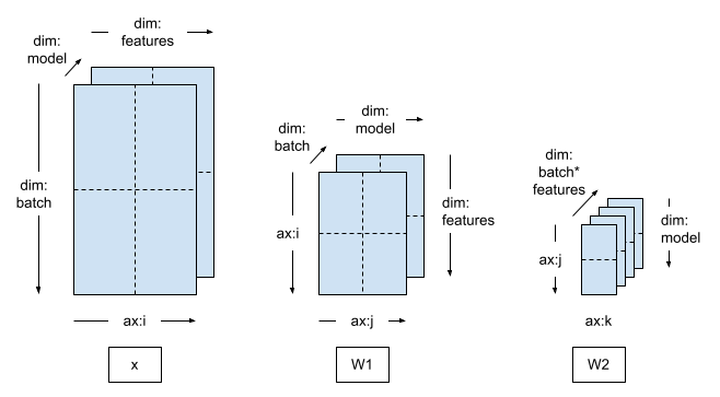
DTensor also supports this case. The only change you need to do is to create a Mesh that includes a feature dimension, and apply the corresponding Layout.
mesh = dtensor.create_mesh([("batch", 2), ("feature", 2), ("model", 2)], devices=DEVICES)
model = MLP([dtensor.Layout(["feature", "model"], mesh),
             dtensor.Layout(["model", dtensor.UNSHARDED], mesh)])
Shard the input data along the feature dimension when packing the input tensors to DTensors. You do this with a slightly different repack function, repack_batch_for_spt, where spt stands for Spatial Parallel Training.
def repack_batch_for_spt(x, y, mesh):
    # Shard data on feature dimension, too
    x = repack_local_tensor(x, layout=dtensor.Layout(["batch", 'feature'], mesh))
    y = repack_local_tensor(y, layout=dtensor.Layout(["batch"], mesh))
    return x, y
The Spatial parallel training can also continue from a checkpoint created with other parallell training schemes.
num_epochs = 2

manager = start_checkpoint_manager(model)
for epoch in range(num_epochs):
  step = 0
  metrics = {'epoch': epoch}
  pbar = tf.keras.utils.Progbar(target=int(train_data_vec.cardinality()))

  for x, y in train_data_vec:
    x, y = repack_batch_for_spt(x, y, mesh)
    metrics.update(train_step(model, x, y, 1e-2))

    pbar.update(step, values=metrics.items(), finalize=False)
    step += 1
  manager.save()
  pbar.update(step, values=metrics.items(), finalize=True)
SavedModel and DTensor
The integration of DTensor and SavedModel is still under development.
As of TensorFlow 2.11, tf.saved_model can save sharded and replicated DTensor models, and saving will do an efficient sharded save on different devices of the mesh. However, after a model is saved, all DTensor annotations are lost and the saved signatures can only be used with regular Tensors, not DTensors.
mesh = dtensor.create_mesh([("world", 1)], devices=DEVICES[:1])
mlp = MLP([dtensor.Layout([dtensor.UNSHARDED, dtensor.UNSHARDED], mesh),
           dtensor.Layout([dtensor.UNSHARDED, dtensor.UNSHARDED], mesh)])

manager = start_checkpoint_manager(mlp)

model_for_saving = tf.keras.Sequential([
  text_vectorization,
  mlp
])

@tf.function(input_signature=[tf.TensorSpec([None], tf.string)])
def run(inputs):
  return {'result': model_for_saving(inputs)}

tf.saved_model.save(
    model_for_saving, "/tmp/saved_model",
    signatures=run)
As of TensorFlow 2.9.0, you can only call a loaded signature with a regular Tensor, or a fully replicated DTensor (which will be converted to a regular Tensor).
sample_batch = train_data.take(1).get_single_element()
sample_batch
loaded = tf.saved_model.load("/tmp/saved_model")

run_sig = loaded.signatures["serving_default"]
result = run_sig(sample_batch['text'])['result']
np.mean(tf.argmax(result, axis=-1) == sample_batch['label'])
What's next?
This tutorial demonstrated building and training an MLP sentiment analysis model with DTensor.
Through Mesh and Layout primitives, DTensor can transform a TensorFlow tf.function to a distributed program suitable for a variety of training schemes.
In a real-world machine learning application, evaluation and cross-validation should be applied to avoid producing an over-fitted model. The techniques introduced in this tutorial can also be applied to introduce parallelism to evaluation.
Composing a model with tf.Module from scratch is a lot of work, and reusing existing building blocks such as layers and helper functions can drastically speed up model development.
As of TensorFlow 2.9, all Keras Layers under tf.keras.layers accepts DTensor layouts as their arguments, and can be used to build DTensor models. You can even directly reuse a Keras model with DTensor without modifying the model implementation. Refer to the DTensor Keras Integration Tutorial for information on using DTensor Keras.