TensorFlow가 5월 14일 Google I/O로 돌아왔습니다! 지금 등록하세요

Estimator를 사용하는 부스트 트리

TensorFlow.org에서 보기

Google Colab에서 실행하기

GitHub에서 소스 보기

노트북 다운로드하기

이 튜토리얼은 tf.estimator API와 함께 의사 결정 트리를 사용하여 그래디언트 부스팅 모델을 훈련하기 위한 전체 연습입니다. 부스트 트리 모델은 회귀 및 분류에 가장 널리 사용되고 효과적인 머신러닝 방식 중 하나입니다. 여러(수십, 수백 또는 수천) 트리 모델의 예측을 결합한 조화로운 기법입니다.

부스트 트리 모델은 최소한의 하이퍼 매개변수 튜닝으로 인상적인 성능을 얻을 수 있기 때문에 많은 머신러닝 전문가 사이에서 인기가 있습니다.

titanic 데이터세트 로드하기

여기서는 titanic 데이터세트를 이용하며 (다소 음산한) 목표는 성별, 나이, 등급 등과 같은 특징을 고려하여 승객 생존을 예측하는 것입니다.

import numpy as np
import pandas as pd
from IPython.display import clear_output
from matplotlib import pyplot as plt

# Load dataset.
dftrain = pd.read_csv('https://storage.googleapis.com/tf-datasets/titanic/train.csv')
dfeval = pd.read_csv('https://storage.googleapis.com/tf-datasets/titanic/eval.csv')
y_train = dftrain.pop('survived')
y_eval = dfeval.pop('survived')

import tensorflow as tf
tf.random.set_seed(123)

데이터세트는 훈련 세트와 평가 세트로 구성됩니다.

dftrain 및 y_train은 훈련 세트입니다(모델이 학습에 사용하는 데이터).
이 모델은 eval set , dfeval 및 y_eval을 대상으로 테스트됩니다.

훈련을 위해 다음 특성을 사용합니다.

특성 이름	설명
sex	승객의 성별
age	승객의 나이
n_siblings_spouses	형제 자매 및 파트너 탑승
parch	부모 및 자녀 탑승
fare	승객이 지불한 요금
수업	유람선의 승객 등급
deck	승객이 있었던 갑판
embark_town	승객이 최초 탑승한 지역
alone	승객이 혼자인지 여부

데이터 탐색하기

먼저 일부 데이터를 미리 살펴보고 훈련 세트에 대한 요약 통계를 작성하겠습니다.

dftrain.head()

dftrain.describe()

훈련 및 평가 세트에는 각각 627개와 264개의 예제가 있습니다.

dftrain.shape[0], dfeval.shape[0]

(627, 264)

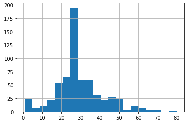
승객의 대다수는 20대와 30대입니다.

dftrain.age.hist(bins=20)
plt.show()

png

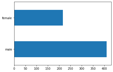
탑승 성별을 보면 여성 승객보다 남성 승객이 약 2배 많습니다.

dftrain.sex.value_counts().plot(kind='barh')
plt.show()

png

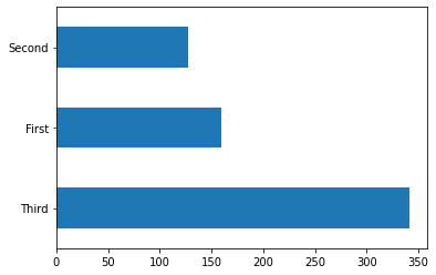
대부분의 승객은 "3등석"에 있었습니다.

dftrain['class'].value_counts().plot(kind='barh')
plt.show()

png

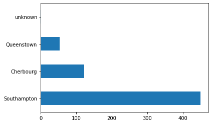
대부분의 승객은 Southampton에서 출발했습니다.

dftrain['embark_town'].value_counts().plot(kind='barh')
plt.show()

png

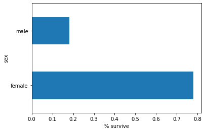
남성보다 여성의 생존 가능성이 훨씬 높습니다. 이 부분은 분명히 모델의 예측 특성이 될 것입니다.

pd.concat([dftrain, y_train], axis=1).groupby('sex').survived.mean().plot(kind='barh').set_xlabel('% survive')
plt.show()

png

특성 열 및 입력 함수 작성하기

그래디언트 부스팅 estimator는 숫자 및 범주별 특성을 모두 사용할 수 있습니다. 특성 열은 모든 TensorFlow estimator에서 작동하며 모델링에 사용되는 특성을 정의하는 것이 목적입니다. 또한 원-핫 인코딩, 정규화 및 버킷화와 같은 몇 가지 특성 엔지니어링 기능도 제공합니다. 이 튜토리얼에서 CATEGORICAL_COLUMNS의 필드는 범주별 열에서 원핫-인코딩된 열(표시기 열)로 변환됩니다.

CATEGORICAL_COLUMNS = ['sex', 'n_siblings_spouses', 'parch', 'class', 'deck',
                       'embark_town', 'alone']
NUMERIC_COLUMNS = ['age', 'fare']

def one_hot_cat_column(feature_name, vocab):
  return tf.feature_column.indicator_column(
      tf.feature_column.categorical_column_with_vocabulary_list(feature_name,
                                                 vocab))
feature_columns = []
for feature_name in CATEGORICAL_COLUMNS:
  # Need to one-hot encode categorical features.
  vocabulary = dftrain[feature_name].unique()
  feature_columns.append(one_hot_cat_column(feature_name, vocabulary))

for feature_name in NUMERIC_COLUMNS:
  feature_columns.append(tf.feature_column.numeric_column(feature_name,
                                           dtype=tf.float32))

특성 열이 생성하는 변환을 볼 수 있습니다. 예를 들어, 단일 예에서 indicator_column을 사용할 때의 출력은 다음과 같습니다.

example = dict(dftrain.head(1))
class_fc = tf.feature_column.indicator_column(tf.feature_column.categorical_column_with_vocabulary_list('class', ('First', 'Second', 'Third')))
print('Feature value: "{}"'.format(example['class'].iloc[0]))
print('One-hot encoded: ', tf.keras.layers.DenseFeatures([class_fc])(example).numpy())

Feature value: "Third"
One-hot encoded:  [[0. 0. 1.]]

또한 모든 특성 열 변환도 함께 볼 수 있습니다.

tf.keras.layers.DenseFeatures(feature_columns)(example).numpy()

array([[22.  ,  1.  ,  0.  ,  1.  ,  0.  ,  0.  ,  1.  ,  0.  ,  0.  ,

         0.  ,  0.  ,  0.  ,  0.  ,  0.  ,  1.  ,  0.  ,  0.  ,  0.  ,
         7.25,  1.  ,  0.  ,  0.  ,  0.  ,  0.  ,  0.  ,  0.  ,  1.  ,
         0.  ,  0.  ,  0.  ,  0.  ,  0.  ,  1.  ,  0.  ]], dtype=float32)

다음으로 입력 함수를 만들어야 합니다. 이 함수는 훈련과 추론을 위해 데이터를 모델로 읽어 들이는 방법을 지정합니다. tf.data API에서 from_tensor_slices 메서드를 사용하여 Pandas에서 직접 데이터를 읽습니다. 이 방법은 작은 인메모리 데이터세트에 적합합니다. 큰 데이터세트의 경우 tf.data API에서 다양한 파일 형식(csv 포함)을 지원하므로 메모리에 맞지 않는 데이터세트를 처리할 수 있습니다.

# Use entire batch since this is such a small dataset.
NUM_EXAMPLES = len(y_train)

def make_input_fn(X, y, n_epochs=None, shuffle=True):
  def input_fn():
    dataset = tf.data.Dataset.from_tensor_slices((dict(X), y))
    if shuffle:
      dataset = dataset.shuffle(NUM_EXAMPLES)
    # For training, cycle thru dataset as many times as need (n_epochs=None).
    dataset = dataset.repeat(n_epochs)
    # In memory training doesn't use batching.
    dataset = dataset.batch(NUM_EXAMPLES)
    return dataset
  return input_fn

# Training and evaluation input functions.
train_input_fn = make_input_fn(dftrain, y_train)
eval_input_fn = make_input_fn(dfeval, y_eval, shuffle=False, n_epochs=1)

모델 훈련 및 평가하기

아래에서 다음 단계를 수행합니다.

특성과 하이퍼 매개변수를 지정하여 모델을 초기화합니다.
train_input_fn을 사용하여 훈련 데이터를 모델에 입력하고 train 함수를 사용하여 모델을 훈련합니다.
평가 세트(이 예에서는 dfeval DataFrame)를 사용하여 모델 성능을 평가합니다. 예측이 y_eval 배열의 레이블과 일치하는지 확인합니다.

부스트 트리 모델을 훈련시키기 전에 먼저 선형 분류자(로지스틱 회귀 모델)를 훈련시켜 보겠습니다. 보다 간단한 모델로 시작하여 벤치마크를 수립하는 것이 가장 좋습니다.

linear_est = tf.estimator.LinearClassifier(feature_columns)

# Train model.
linear_est.train(train_input_fn, max_steps=100)

# Evaluation.
result = linear_est.evaluate(eval_input_fn)
clear_output()
print(pd.Series(result))

accuracy                  0.765152
accuracy_baseline         0.625000
auc                       0.832844
auc_precision_recall      0.789631
average_loss              0.478908
label/mean                0.375000
loss                      0.478908
precision                 0.703297
prediction/mean           0.350790
recall                    0.646465
global_step             100.000000
dtype: float64

다음으로 부스트 트리 모델을 훈련시켜 보겠습니다. 부스트 트리의 경우 회귀(BoostedTreesRegressor) 및 분류(BoostedTreesClassifier)가 지원됩니다. 등급 생존(생존 또는 비생존)을 예측하는 것이 목표이므로 BoostedTreesClassifier를 사용합니다.

# Since data fits into memory, use entire dataset per layer. It will be faster.
# Above one batch is defined as the entire dataset.
n_batches = 1
est = tf.estimator.BoostedTreesClassifier(feature_columns,
                                          n_batches_per_layer=n_batches)

# The model will stop training once the specified number of trees is built, not
# based on the number of steps.
est.train(train_input_fn, max_steps=100)

# Eval.
result = est.evaluate(eval_input_fn)
clear_output()
print(pd.Series(result))

accuracy                  0.833333
accuracy_baseline         0.625000
auc                       0.874778
auc_precision_recall      0.859794
average_loss              0.406492
label/mean                0.375000
loss                      0.406492
precision                 0.795699
prediction/mean           0.385033
recall                    0.747475
global_step             100.000000
dtype: float64

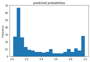
이제 훈련 모델을 사용하여 평가 세트로부터 승객을 예측할 수 있습니다. TensorFlow 모델은 한 번에 여러 예제의 배치나 모음에 대해 예측하도록 최적화되어 있습니다. 이전에는 eval_input_fn이 전체 평가 세트를 사용하여 정의되었습니다.

pred_dicts = list(est.predict(eval_input_fn))
probs = pd.Series([pred['probabilities'][1] for pred in pred_dicts])

probs.plot(kind='hist', bins=20, title='predicted probabilities')
plt.show()

INFO:tensorflow:Calling model_fn.
INFO:tensorflow:Done calling model_fn.
INFO:tensorflow:Graph was finalized.
INFO:tensorflow:Restoring parameters from /tmp/tmpuhlub0wq/model.ckpt-100
INFO:tensorflow:Running local_init_op.
INFO:tensorflow:Done running local_init_op.

png

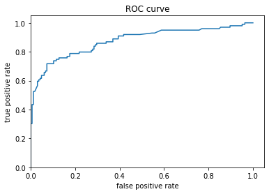
마지막으로, 결과의 ROC(Receiver operating characteristic)도 볼 수 있습니다. 이로부터 참양성률과 거짓양성률 간의 상충 관계에 대한 더 나은 개념을 얻을 수 있습니다.

from sklearn.metrics import roc_curve

fpr, tpr, _ = roc_curve(y_eval, probs)
plt.plot(fpr, tpr)
plt.title('ROC curve')
plt.xlabel('false positive rate')
plt.ylabel('true positive rate')
plt.xlim(0,)
plt.ylim(0,)
plt.show()

png