
|
|
|
 View source on GitHub
|
|
This tutorial focuses on the task of image segmentation, using a modified U-Net.
What is image segmentation?
In an image classification task, the network assigns a label (or class) to each input image. However, suppose you want to know the shape of that object, which pixel belongs to which object, etc. In this case, you need to assign a class to each pixel of the image—this task is known as segmentation. A segmentation model returns much more detailed information about the image. Image segmentation has many applications in medical imaging, self-driving cars and satellite imaging, just to name a few.
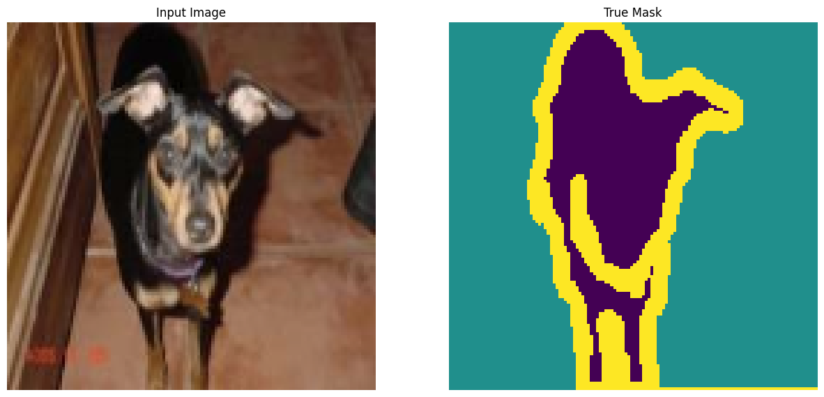
This tutorial uses the Oxford-IIIT Pet Dataset (Parkhi et al, 2012). The dataset consists of images of 37 pet breeds, with 200 images per breed (~100 each in the training and test splits). Each image includes the corresponding labels, and pixel-wise masks. The masks are class-labels for each pixel. Each pixel is given one of three categories:
- Class 1: Pixel belonging to the pet.
- Class 2: Pixel bordering the pet.
- Class 3: None of the above/a surrounding pixel.
pip install git+https://github.com/tensorflow/examples.gitpip install -U keraspip install -q tensorflow_datasetspip install -q -U tensorflow-text tensorflow
import numpy as np

import tensorflow as tf
import tensorflow_datasets as tfds
2024-08-16 03:11:30.435396: E external/local_xla/xla/stream_executor/cuda/cuda_fft.cc:485] Unable to register cuFFT factory: Attempting to register factory for plugin cuFFT when one has already been registered
2024-08-16 03:11:30.457043: E external/local_xla/xla/stream_executor/cuda/cuda_dnn.cc:8454] Unable to register cuDNN factory: Attempting to register factory for plugin cuDNN when one has already been registered
2024-08-16 03:11:30.463367: E external/local_xla/xla/stream_executor/cuda/cuda_blas.cc:1452] Unable to register cuBLAS factory: Attempting to register factory for plugin cuBLAS when one has already been registered
from tensorflow_examples.models.pix2pix import pix2pix

from IPython.display import clear_output
import matplotlib.pyplot as plt
Download the Oxford-IIIT Pets dataset
The dataset is available from TensorFlow Datasets. The segmentation masks are included in version 3+.
dataset, info = tfds.load('oxford_iiit_pet:3.*.*', with_info=True)
WARNING: All log messages before absl::InitializeLog() is called are written to STDERR
I0000 00:00:1723777894.956816  128784 cuda_executor.cc:1015] successful NUMA node read from SysFS had negative value (-1), but there must be at least one NUMA node, so returning NUMA node zero. See more at https://github.com/torvalds/linux/blob/v6.0/Documentation/ABI/testing/sysfs-bus-pci#L344-L355
I0000 00:00:1723777894.960610  128784 cuda_executor.cc:1015] successful NUMA node read from SysFS had negative value (-1), but there must be at least one NUMA node, so returning NUMA node zero. See more at https://github.com/torvalds/linux/blob/v6.0/Documentation/ABI/testing/sysfs-bus-pci#L344-L355
I0000 00:00:1723777894.964173  128784 cuda_executor.cc:1015] successful NUMA node read from SysFS had negative value (-1), but there must be at least one NUMA node, so returning NUMA node zero. See more at https://github.com/torvalds/linux/blob/v6.0/Documentation/ABI/testing/sysfs-bus-pci#L344-L355
I0000 00:00:1723777894.967995  128784 cuda_executor.cc:1015] successful NUMA node read from SysFS had negative value (-1), but there must be at least one NUMA node, so returning NUMA node zero. See more at https://github.com/torvalds/linux/blob/v6.0/Documentation/ABI/testing/sysfs-bus-pci#L344-L355
I0000 00:00:1723777894.979249  128784 cuda_executor.cc:1015] successful NUMA node read from SysFS had negative value (-1), but there must be at least one NUMA node, so returning NUMA node zero. See more at https://github.com/torvalds/linux/blob/v6.0/Documentation/ABI/testing/sysfs-bus-pci#L344-L355
I0000 00:00:1723777894.982762  128784 cuda_executor.cc:1015] successful NUMA node read from SysFS had negative value (-1), but there must be at least one NUMA node, so returning NUMA node zero. See more at https://github.com/torvalds/linux/blob/v6.0/Documentation/ABI/testing/sysfs-bus-pci#L344-L355
I0000 00:00:1723777894.986159  128784 cuda_executor.cc:1015] successful NUMA node read from SysFS had negative value (-1), but there must be at least one NUMA node, so returning NUMA node zero. See more at https://github.com/torvalds/linux/blob/v6.0/Documentation/ABI/testing/sysfs-bus-pci#L344-L355
I0000 00:00:1723777894.989705  128784 cuda_executor.cc:1015] successful NUMA node read from SysFS had negative value (-1), but there must be at least one NUMA node, so returning NUMA node zero. See more at https://github.com/torvalds/linux/blob/v6.0/Documentation/ABI/testing/sysfs-bus-pci#L344-L355
I0000 00:00:1723777894.993180  128784 cuda_executor.cc:1015] successful NUMA node read from SysFS had negative value (-1), but there must be at least one NUMA node, so returning NUMA node zero. See more at https://github.com/torvalds/linux/blob/v6.0/Documentation/ABI/testing/sysfs-bus-pci#L344-L355
I0000 00:00:1723777894.996611  128784 cuda_executor.cc:1015] successful NUMA node read from SysFS had negative value (-1), but there must be at least one NUMA node, so returning NUMA node zero. See more at https://github.com/torvalds/linux/blob/v6.0/Documentation/ABI/testing/sysfs-bus-pci#L344-L355
I0000 00:00:1723777894.999909  128784 cuda_executor.cc:1015] successful NUMA node read from SysFS had negative value (-1), but there must be at least one NUMA node, so returning NUMA node zero. See more at https://github.com/torvalds/linux/blob/v6.0/Documentation/ABI/testing/sysfs-bus-pci#L344-L355
I0000 00:00:1723777895.003335  128784 cuda_executor.cc:1015] successful NUMA node read from SysFS had negative value (-1), but there must be at least one NUMA node, so returning NUMA node zero. See more at https://github.com/torvalds/linux/blob/v6.0/Documentation/ABI/testing/sysfs-bus-pci#L344-L355
I0000 00:00:1723777896.245027  128784 cuda_executor.cc:1015] successful NUMA node read from SysFS had negative value (-1), but there must be at least one NUMA node, so returning NUMA node zero. See more at https://github.com/torvalds/linux/blob/v6.0/Documentation/ABI/testing/sysfs-bus-pci#L344-L355
I0000 00:00:1723777896.247086  128784 cuda_executor.cc:1015] successful NUMA node read from SysFS had negative value (-1), but there must be at least one NUMA node, so returning NUMA node zero. See more at https://github.com/torvalds/linux/blob/v6.0/Documentation/ABI/testing/sysfs-bus-pci#L344-L355
I0000 00:00:1723777896.249144  128784 cuda_executor.cc:1015] successful NUMA node read from SysFS had negative value (-1), but there must be at least one NUMA node, so returning NUMA node zero. See more at https://github.com/torvalds/linux/blob/v6.0/Documentation/ABI/testing/sysfs-bus-pci#L344-L355
I0000 00:00:1723777896.251246  128784 cuda_executor.cc:1015] successful NUMA node read from SysFS had negative value (-1), but there must be at least one NUMA node, so returning NUMA node zero. See more at https://github.com/torvalds/linux/blob/v6.0/Documentation/ABI/testing/sysfs-bus-pci#L344-L355
I0000 00:00:1723777896.253265  128784 cuda_executor.cc:1015] successful NUMA node read from SysFS had negative value (-1), but there must be at least one NUMA node, so returning NUMA node zero. See more at https://github.com/torvalds/linux/blob/v6.0/Documentation/ABI/testing/sysfs-bus-pci#L344-L355
I0000 00:00:1723777896.255177  128784 cuda_executor.cc:1015] successful NUMA node read from SysFS had negative value (-1), but there must be at least one NUMA node, so returning NUMA node zero. See more at https://github.com/torvalds/linux/blob/v6.0/Documentation/ABI/testing/sysfs-bus-pci#L344-L355
I0000 00:00:1723777896.257133  128784 cuda_executor.cc:1015] successful NUMA node read from SysFS had negative value (-1), but there must be at least one NUMA node, so returning NUMA node zero. See more at https://github.com/torvalds/linux/blob/v6.0/Documentation/ABI/testing/sysfs-bus-pci#L344-L355
I0000 00:00:1723777896.259176  128784 cuda_executor.cc:1015] successful NUMA node read from SysFS had negative value (-1), but there must be at least one NUMA node, so returning NUMA node zero. See more at https://github.com/torvalds/linux/blob/v6.0/Documentation/ABI/testing/sysfs-bus-pci#L344-L355
I0000 00:00:1723777896.261081  128784 cuda_executor.cc:1015] successful NUMA node read from SysFS had negative value (-1), but there must be at least one NUMA node, so returning NUMA node zero. See more at https://github.com/torvalds/linux/blob/v6.0/Documentation/ABI/testing/sysfs-bus-pci#L344-L355
I0000 00:00:1723777896.262978  128784 cuda_executor.cc:1015] successful NUMA node read from SysFS had negative value (-1), but there must be at least one NUMA node, so returning NUMA node zero. See more at https://github.com/torvalds/linux/blob/v6.0/Documentation/ABI/testing/sysfs-bus-pci#L344-L355
I0000 00:00:1723777896.264935  128784 cuda_executor.cc:1015] successful NUMA node read from SysFS had negative value (-1), but there must be at least one NUMA node, so returning NUMA node zero. See more at https://github.com/torvalds/linux/blob/v6.0/Documentation/ABI/testing/sysfs-bus-pci#L344-L355
I0000 00:00:1723777896.267032  128784 cuda_executor.cc:1015] successful NUMA node read from SysFS had negative value (-1), but there must be at least one NUMA node, so returning NUMA node zero. See more at https://github.com/torvalds/linux/blob/v6.0/Documentation/ABI/testing/sysfs-bus-pci#L344-L355
I0000 00:00:1723777896.304992  128784 cuda_executor.cc:1015] successful NUMA node read from SysFS had negative value (-1), but there must be at least one NUMA node, so returning NUMA node zero. See more at https://github.com/torvalds/linux/blob/v6.0/Documentation/ABI/testing/sysfs-bus-pci#L344-L355
I0000 00:00:1723777896.306981  128784 cuda_executor.cc:1015] successful NUMA node read from SysFS had negative value (-1), but there must be at least one NUMA node, so returning NUMA node zero. See more at https://github.com/torvalds/linux/blob/v6.0/Documentation/ABI/testing/sysfs-bus-pci#L344-L355
I0000 00:00:1723777896.308981  128784 cuda_executor.cc:1015] successful NUMA node read from SysFS had negative value (-1), but there must be at least one NUMA node, so returning NUMA node zero. See more at https://github.com/torvalds/linux/blob/v6.0/Documentation/ABI/testing/sysfs-bus-pci#L344-L355
I0000 00:00:1723777896.311004  128784 cuda_executor.cc:1015] successful NUMA node read from SysFS had negative value (-1), but there must be at least one NUMA node, so returning NUMA node zero. See more at https://github.com/torvalds/linux/blob/v6.0/Documentation/ABI/testing/sysfs-bus-pci#L344-L355
I0000 00:00:1723777896.312927  128784 cuda_executor.cc:1015] successful NUMA node read from SysFS had negative value (-1), but there must be at least one NUMA node, so returning NUMA node zero. See more at https://github.com/torvalds/linux/blob/v6.0/Documentation/ABI/testing/sysfs-bus-pci#L344-L355
I0000 00:00:1723777896.314851  128784 cuda_executor.cc:1015] successful NUMA node read from SysFS had negative value (-1), but there must be at least one NUMA node, so returning NUMA node zero. See more at https://github.com/torvalds/linux/blob/v6.0/Documentation/ABI/testing/sysfs-bus-pci#L344-L355
I0000 00:00:1723777896.316803  128784 cuda_executor.cc:1015] successful NUMA node read from SysFS had negative value (-1), but there must be at least one NUMA node, so returning NUMA node zero. See more at https://github.com/torvalds/linux/blob/v6.0/Documentation/ABI/testing/sysfs-bus-pci#L344-L355
I0000 00:00:1723777896.318808  128784 cuda_executor.cc:1015] successful NUMA node read from SysFS had negative value (-1), but there must be at least one NUMA node, so returning NUMA node zero. See more at https://github.com/torvalds/linux/blob/v6.0/Documentation/ABI/testing/sysfs-bus-pci#L344-L355
I0000 00:00:1723777896.320732  128784 cuda_executor.cc:1015] successful NUMA node read from SysFS had negative value (-1), but there must be at least one NUMA node, so returning NUMA node zero. See more at https://github.com/torvalds/linux/blob/v6.0/Documentation/ABI/testing/sysfs-bus-pci#L344-L355
I0000 00:00:1723777896.323004  128784 cuda_executor.cc:1015] successful NUMA node read from SysFS had negative value (-1), but there must be at least one NUMA node, so returning NUMA node zero. See more at https://github.com/torvalds/linux/blob/v6.0/Documentation/ABI/testing/sysfs-bus-pci#L344-L355
I0000 00:00:1723777896.325324  128784 cuda_executor.cc:1015] successful NUMA node read from SysFS had negative value (-1), but there must be at least one NUMA node, so returning NUMA node zero. See more at https://github.com/torvalds/linux/blob/v6.0/Documentation/ABI/testing/sysfs-bus-pci#L344-L355
I0000 00:00:1723777896.327769  128784 cuda_executor.cc:1015] successful NUMA node read from SysFS had negative value (-1), but there must be at least one NUMA node, so returning NUMA node zero. See more at https://github.com/torvalds/linux/blob/v6.0/Documentation/ABI/testing/sysfs-bus-pci#L344-L355
In addition, the image color values are normalized to the [0, 1] range. Finally, as mentioned above the pixels in the segmentation mask are labeled either {1, 2, 3}. For the sake of convenience, subtract 1 from the segmentation mask, resulting in labels that are : {0, 1, 2}.
def normalize(input_image, input_mask):
  input_image = tf.cast(input_image, tf.float32) / 255.0
  input_mask -= 1
  return input_image, input_mask
def load_image(datapoint):
  input_image = tf.image.resize(datapoint['image'], (128, 128))
  input_mask = tf.image.resize(
    datapoint['segmentation_mask'],
    (128, 128),
    method = tf.image.ResizeMethod.NEAREST_NEIGHBOR,
  )

  input_image, input_mask = normalize(input_image, input_mask)

  return input_image, input_mask
The dataset already contains the required training and test splits, so continue to use the same splits:
TRAIN_LENGTH = info.splits['train'].num_examples
BATCH_SIZE = 64
BUFFER_SIZE = 1000
STEPS_PER_EPOCH = TRAIN_LENGTH // BATCH_SIZE
train_images = dataset['train'].map(load_image, num_parallel_calls=tf.data.AUTOTUNE)
test_images = dataset['test'].map(load_image, num_parallel_calls=tf.data.AUTOTUNE)
The following class performs a simple augmentation by randomly-flipping an image. Go to the Image augmentation tutorial to learn more.
class Augment(tf.keras.layers.Layer):
  def __init__(self, seed=42):
    super().__init__()
    # both use the same seed, so they'll make the same random changes.
    self.augment_inputs = tf.keras.layers.RandomFlip(mode="horizontal", seed=seed)
    self.augment_labels = tf.keras.layers.RandomFlip(mode="horizontal", seed=seed)

  def call(self, inputs, labels):
    inputs = self.augment_inputs(inputs)
    labels = self.augment_labels(labels)
    return inputs, labels
Build the input pipeline, applying the augmentation after batching the inputs:
train_batches = (
    train_images
    .cache()
    .shuffle(BUFFER_SIZE)
    .batch(BATCH_SIZE)
    .repeat()
    .map(Augment())
    .prefetch(buffer_size=tf.data.AUTOTUNE))

test_batches = test_images.batch(BATCH_SIZE)
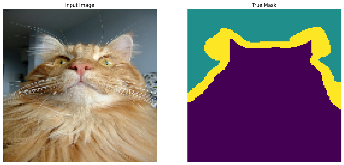
Visualize an image example and its corresponding mask from the dataset:
def display(display_list):
  plt.figure(figsize=(15, 15))

  title = ['Input Image', 'True Mask', 'Predicted Mask']

  for i in range(len(display_list)):
    plt.subplot(1, len(display_list), i+1)
    plt.title(title[i])
    plt.imshow(tf.keras.utils.array_to_img(display_list[i]))
    plt.axis('off')
  plt.show()
for images, masks in train_batches.take(2):
  sample_image, sample_mask = images[0], masks[0]
  display([sample_image, sample_mask])
Corrupt JPEG data: 240 extraneous bytes before marker 0xd9
Corrupt JPEG data: premature end of data segment
2024-08-16 03:11:39.796476: W tensorflow/core/kernels/data/cache_dataset_ops.cc:913] The calling iterator did not fully read the dataset being cached. In order to avoid unexpected truncation of the dataset, the partially cached contents of the dataset will be discarded. This can happen if you have an input pipeline similar to `dataset.cache().take(k).repeat()`. You should use `dataset.take(k).cache().repeat()` instead.
Define the model
The model being used here is a modified U-Net. A U-Net consists of an encoder (downsampler) and decoder (upsampler). To learn robust features and reduce the number of trainable parameters, use a pretrained model—MobileNetV2—as the encoder. For the decoder, you will use the upsample block, which is already implemented in the pix2pix example in the TensorFlow Examples repo. (Check out the pix2pix: Image-to-image translation with a conditional GAN tutorial in a notebook.)
As mentioned, the encoder is a pretrained MobileNetV2 model. You will use the model from tf.keras.applications. The encoder consists of specific outputs from intermediate layers in the model. Note that the encoder will not be trained during the training process.
base_model = tf.keras.applications.MobileNetV2(input_shape=[128, 128, 3], include_top=False)

# Use the activations of these layers
layer_names = [
    'block_1_expand_relu',   # 64x64
    'block_3_expand_relu',   # 32x32
    'block_6_expand_relu',   # 16x16
    'block_13_expand_relu',  # 8x8
    'block_16_project',      # 4x4
]
base_model_outputs = [base_model.get_layer(name).output for name in layer_names]

# Create the feature extraction model
down_stack = tf.keras.Model(inputs=base_model.input, outputs=base_model_outputs)

down_stack.trainable = False
Downloading data from https://storage.googleapis.com/tensorflow/keras-applications/mobilenet_v2/mobilenet_v2_weights_tf_dim_ordering_tf_kernels_1.0_128_no_top.h5
9406464/9406464 ━━━━━━━━━━━━━━━━━━━━ 0s 0us/step
The decoder/upsampler is simply a series of upsample blocks implemented in TensorFlow examples:
up_stack = [
    pix2pix.upsample(512, 3),  # 4x4 -> 8x8
    pix2pix.upsample(256, 3),  # 8x8 -> 16x16
    pix2pix.upsample(128, 3),  # 16x16 -> 32x32
    pix2pix.upsample(64, 3),   # 32x32 -> 64x64
]
def unet_model(output_channels:int):
  inputs = tf.keras.layers.Input(shape=[128, 128, 3])

  # Downsampling through the model
  skips = down_stack(inputs)
  x = skips[-1]
  skips = reversed(skips[:-1])

  # Upsampling and establishing the skip connections
  for up, skip in zip(up_stack, skips):
    x = up(x)
    concat = tf.keras.layers.Concatenate()
    x = concat([x, skip])

  # This is the last layer of the model
  last = tf.keras.layers.Conv2DTranspose(
      filters=output_channels, kernel_size=3, strides=2,
      padding='same')  #64x64 -> 128x128

  x = last(x)

  return tf.keras.Model(inputs=inputs, outputs=x)
Note that the number of filters on the last layer is set to the number of output_channels. This will be one output channel per class.
Train the model
Now, all that is left to do is to compile and train the model.
Since this is a multiclass classification problem, use the tf.keras.losses.SparseCategoricalCrossentropy loss function with the from_logits argument set to True, since the labels are scalar integers instead of vectors of scores for each pixel of every class.
When running inference, the label assigned to the pixel is the channel with the highest value. This is what the create_mask function is doing.
OUTPUT_CLASSES = 3

model = unet_model(output_channels=OUTPUT_CLASSES)
model.compile(optimizer='adam',
              loss=tf.keras.losses.SparseCategoricalCrossentropy(from_logits=True),
              metrics=['accuracy'])
Plot the resulting model architecture:
tf.keras.utils.plot_model(model, show_shapes=True, expand_nested=True, dpi=64)

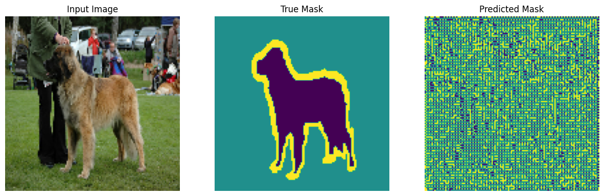
Try out the model to check what it predicts before training:
def create_mask(pred_mask):
  pred_mask = tf.math.argmax(pred_mask, axis=-1)
  pred_mask = pred_mask[..., tf.newaxis]
  return pred_mask[0]
def show_predictions(dataset=None, num=1):
  if dataset:
    for image, mask in dataset.take(num):
      pred_mask = model.predict(image)
      display([image[0], mask[0], create_mask(pred_mask)])
  else:
    display([sample_image, sample_mask,
             create_mask(model.predict(sample_image[tf.newaxis, ...]))])
show_predictions()
WARNING: All log messages before absl::InitializeLog() is called are written to STDERR
I0000 00:00:1723777904.241553  129005 service.cc:146] XLA service 0x7f02cc001640 initialized for platform CUDA (this does not guarantee that XLA will be used). Devices:
I0000 00:00:1723777904.241587  129005 service.cc:154]   StreamExecutor device (0): Tesla T4, Compute Capability 7.5
I0000 00:00:1723777904.241591  129005 service.cc:154]   StreamExecutor device (1): Tesla T4, Compute Capability 7.5
I0000 00:00:1723777904.241593  129005 service.cc:154]   StreamExecutor device (2): Tesla T4, Compute Capability 7.5
I0000 00:00:1723777904.241596  129005 service.cc:154]   StreamExecutor device (3): Tesla T4, Compute Capability 7.5
1/1 ━━━━━━━━━━━━━━━━━━━━ 4s 4s/step
I0000 00:00:1723777907.244468  129005 device_compiler.h:188] Compiled cluster using XLA!  This line is logged at most once for the lifetime of the process.
The callback defined below is used to observe how the model improves while it is training:
class DisplayCallback(tf.keras.callbacks.Callback):
  def on_epoch_end(self, epoch, logs=None):
    clear_output(wait=True)
    show_predictions()
    print ('\nSample Prediction after epoch {}\n'.format(epoch+1))
EPOCHS = 20
VAL_SUBSPLITS = 5
VALIDATION_STEPS = info.splits['test'].num_examples//BATCH_SIZE//VAL_SUBSPLITS

model_history = model.fit(train_batches, epochs=EPOCHS,
                          steps_per_epoch=STEPS_PER_EPOCH,
                          validation_steps=VALIDATION_STEPS,
                          validation_data=test_batches,
                          callbacks=[DisplayCallback()])
1/1 ━━━━━━━━━━━━━━━━━━━━ 0s 44ms/step
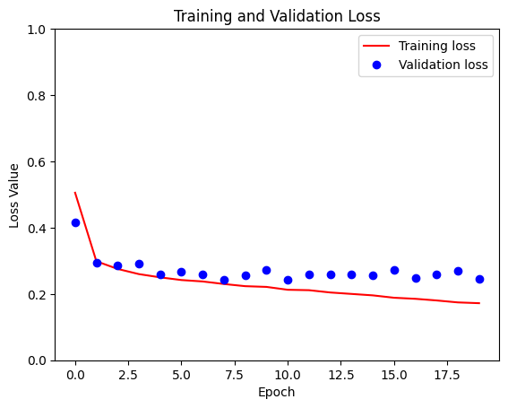
Sample Prediction after epoch 20

57/57 ━━━━━━━━━━━━━━━━━━━━ 8s 137ms/step - accuracy: 0.9285 - loss: 0.1754 - val_accuracy: 0.9076 - val_loss: 0.2465
loss = model_history.history['loss']
val_loss = model_history.history['val_loss']

plt.figure()
plt.plot(model_history.epoch, loss, 'r', label='Training loss')
plt.plot(model_history.epoch, val_loss, 'bo', label='Validation loss')
plt.title('Training and Validation Loss')
plt.xlabel('Epoch')
plt.ylabel('Loss Value')
plt.ylim([0, 1])
plt.legend()
plt.show()
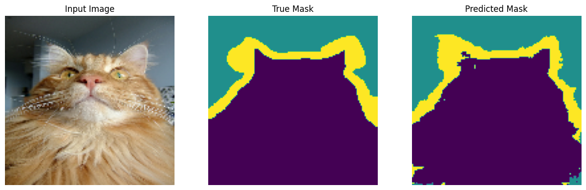
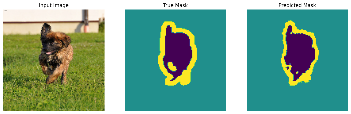
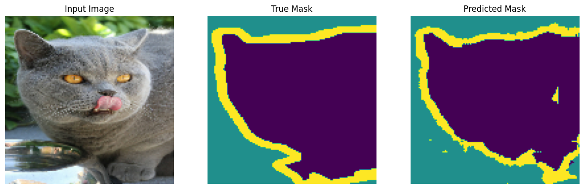
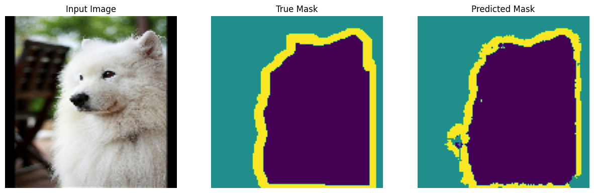
Make predictions
Now, make some predictions. In the interest of saving time, the number of epochs was kept small, but you may set this higher to achieve more accurate results.
show_predictions(test_batches, 3)
2/2 ━━━━━━━━━━━━━━━━━━━━ 2s 25ms/step
2/2 ━━━━━━━━━━━━━━━━━━━━ 0s 35ms/step
2/2 ━━━━━━━━━━━━━━━━━━━━ 0s 35ms/step
Optional: Imbalanced classes and class weights
Semantic segmentation datasets can be highly imbalanced meaning that particular class pixels can be present more inside images than that of other classes. Since segmentation problems can be treated as per-pixel classification problems, you can deal with the imbalance problem by weighing the loss function to account for this. It's a simple and elegant way to deal with this problem. Refer to the Classification on imbalanced data tutorial to learn more.
To avoid ambiguity, Model.fit does not support the class_weight argument for targets with 3+ dimensions.
try:
  model_history = model.fit(train_batches, epochs=EPOCHS,
                            steps_per_epoch=STEPS_PER_EPOCH,
                            class_weight = {0:2.0, 1:2.0, 2:1.0})
  assert False
except Exception as e:
  print(f"Expected {type(e).__name__}: {e}")
Epoch 1/20
W0000 00:00:1723778113.501185  129000 assert_op.cc:38] Ignoring Assert operator compile_loss/sparse_categorical_crossentropy/SparseSoftmaxCrossEntropyWithLogits/assert_equal_1/Assert/Assert
57/57 ━━━━━━━━━━━━━━━━━━━━ 13s 113ms/step - accuracy: 0.9249 - loss: 0.2495
Epoch 2/20
W0000 00:00:1723778123.461684  129003 assert_op.cc:38] Ignoring Assert operator compile_loss/sparse_categorical_crossentropy/SparseSoftmaxCrossEntropyWithLogits/assert_equal_1/Assert/Assert
57/57 ━━━━━━━━━━━━━━━━━━━━ 10s 119ms/step - accuracy: 0.9231 - loss: 0.2522
Epoch 3/20
57/57 ━━━━━━━━━━━━━━━━━━━━ 7s 120ms/step - accuracy: 0.9261 - loss: 0.2397
Epoch 4/20
57/57 ━━━━━━━━━━━━━━━━━━━━ 7s 121ms/step - accuracy: 0.9272 - loss: 0.2349
Epoch 5/20
57/57 ━━━━━━━━━━━━━━━━━━━━ 7s 129ms/step - accuracy: 0.9301 - loss: 0.2237
Epoch 6/20
57/57 ━━━━━━━━━━━━━━━━━━━━ 7s 124ms/step - accuracy: 0.9323 - loss: 0.2167
Epoch 7/20
57/57 ━━━━━━━━━━━━━━━━━━━━ 7s 120ms/step - accuracy: 0.9352 - loss: 0.2060
Epoch 8/20
57/57 ━━━━━━━━━━━━━━━━━━━━ 7s 120ms/step - accuracy: 0.9347 - loss: 0.2068
Epoch 9/20
57/57 ━━━━━━━━━━━━━━━━━━━━ 7s 119ms/step - accuracy: 0.9382 - loss: 0.1946
Epoch 10/20
57/57 ━━━━━━━━━━━━━━━━━━━━ 7s 115ms/step - accuracy: 0.9391 - loss: 0.1902
Epoch 11/20
57/57 ━━━━━━━━━━━━━━━━━━━━ 6s 114ms/step - accuracy: 0.9394 - loss: 0.1895
Epoch 12/20
57/57 ━━━━━━━━━━━━━━━━━━━━ 6s 113ms/step - accuracy: 0.9406 - loss: 0.1864
Epoch 13/20
57/57 ━━━━━━━━━━━━━━━━━━━━ 6s 114ms/step - accuracy: 0.9412 - loss: 0.1845
Epoch 14/20
57/57 ━━━━━━━━━━━━━━━━━━━━ 7s 116ms/step - accuracy: 0.9440 - loss: 0.1740
Epoch 15/20
57/57 ━━━━━━━━━━━━━━━━━━━━ 7s 119ms/step - accuracy: 0.9462 - loss: 0.1665
Epoch 16/20
57/57 ━━━━━━━━━━━━━━━━━━━━ 7s 120ms/step - accuracy: 0.9465 - loss: 0.1667
Epoch 17/20
57/57 ━━━━━━━━━━━━━━━━━━━━ 7s 120ms/step - accuracy: 0.9471 - loss: 0.1639
Epoch 18/20
57/57 ━━━━━━━━━━━━━━━━━━━━ 7s 120ms/step - accuracy: 0.9491 - loss: 0.1560
Epoch 19/20
57/57 ━━━━━━━━━━━━━━━━━━━━ 7s 120ms/step - accuracy: 0.9495 - loss: 0.1561
Epoch 20/20
57/57 ━━━━━━━━━━━━━━━━━━━━ 7s 120ms/step - accuracy: 0.9505 - loss: 0.1533
Expected AssertionError:
So, in this case you need to implement the weighting yourself. You'll do this using sample weights: In addition to (data, label) pairs, Model.fit also accepts (data, label, sample_weight) triples.
Keras Model.fit propagates the sample_weight to the losses and metrics, which also accept a sample_weight argument. The sample weight is multiplied by the sample's value before the reduction step. For example:
label = np.array([0,0])
prediction = np.array([[-3., 0], [-3, 0]])
sample_weight = [1, 10]

loss = tf.keras.losses.SparseCategoricalCrossentropy(
    from_logits=True,
    reduction=tf.keras.losses.Reduction.NONE
)
loss(label, prediction, sample_weight).numpy()
array([ 3.0485873, 30.485874 ], dtype=float32)
So, to make sample weights for this tutorial, you need a function that takes a (data, label) pair and returns a (data, label, sample_weight) triple where the sample_weight is a 1-channel image containing the class weight for each pixel.
The simplest possible implementation is to use the label as an index into a class_weight list:
def add_sample_weights(image, label):
  # The weights for each class, with the constraint that:
  #     sum(class_weights) == 1.0
  class_weights = tf.constant([2.0, 2.0, 1.0])
  class_weights = class_weights/tf.reduce_sum(class_weights)

  # Create an image of `sample_weights` by using the label at each pixel as an
  # index into the `class weights` .
  sample_weights = tf.gather(class_weights, indices=tf.cast(label, tf.int32))

  return image, label, sample_weights
The resulting dataset elements contain 3 images each:
train_batches.map(add_sample_weights).element_spec
(TensorSpec(shape=(None, 128, 128, 3), dtype=tf.float32, name=None),
 TensorSpec(shape=(None, 128, 128, 1), dtype=tf.float32, name=None),
 TensorSpec(shape=(None, 128, 128, 1), dtype=tf.float32, name=None))
Now, you can train a model on this weighted dataset:
weighted_model = unet_model(OUTPUT_CLASSES)
weighted_model.compile(
    optimizer='adam',
    loss=tf.keras.losses.SparseCategoricalCrossentropy(from_logits=True),
    metrics=['accuracy'])
weighted_model.fit(
    train_batches.map(add_sample_weights),
    epochs=1,
    steps_per_epoch=10)
W0000 00:00:1723778261.427975  129000 assert_op.cc:38] Ignoring Assert operator compile_loss/sparse_categorical_crossentropy/SparseSoftmaxCrossEntropyWithLogits/assert_equal_1/Assert/Assert
10/10 ━━━━━━━━━━━━━━━━━━━━ 9s 113ms/step - accuracy: 0.4253 - loss: 0.4664
<keras.src.callbacks.history.History at 0x7f041c2a12b0>
Next steps
Now that you have an understanding of what image segmentation is and how it works, you can try this tutorial out with different intermediate layer outputs, or even different pretrained models. You may also challenge yourself by trying out the Carvana image masking challenge hosted on Kaggle.
You may also want to see the Tensorflow Object Detection API for another model you can retrain on your own data. Pretrained models are available on TensorFlow Hub.