
 View on TensorFlow.org |
 Run in Google Colab |
 View source on GitHub |
 Download notebook |
In a regression problem, the aim is to predict the output of a continuous value, like a price or a probability. Contrast this with a classification problem, where the aim is to select a class from a list of classes (for example, where a picture contains an apple or an orange, recognizing which fruit is in the picture).
This tutorial uses the classic Auto MPG dataset and demonstrates how to build models to predict the fuel efficiency of the late-1970s and early 1980s automobiles. To do this, you will provide the models with a description of many automobiles from that time period. This description includes attributes like cylinders, displacement, horsepower, and weight.
This example uses the Keras API. (Visit the Keras tutorials and guides to learn more.)
# Use seaborn for pairplot.pip install -q seaborn
import matplotlib.pyplot as plt
import numpy as np
import pandas as pd
import seaborn as sns

# Make NumPy printouts easier to read.
np.set_printoptions(precision=3, suppress=True)
import tensorflow as tf

from tensorflow import keras
from tensorflow.keras import layers

print(tf.__version__)
2025-12-03 05:26:23.046162: E external/local_xla/xla/stream_executor/cuda/cuda_fft.cc:467] Unable to register cuFFT factory: Attempting to register factory for plugin cuFFT when one has already been registered
WARNING: All log messages before absl::InitializeLog() is called are written to STDERR
E0000 00:00:1764739583.069252  534406 cuda_dnn.cc:8579] Unable to register cuDNN factory: Attempting to register factory for plugin cuDNN when one has already been registered
E0000 00:00:1764739583.076859  534406 cuda_blas.cc:1407] Unable to register cuBLAS factory: Attempting to register factory for plugin cuBLAS when one has already been registered
W0000 00:00:1764739583.095512  534406 computation_placer.cc:177] computation placer already registered. Please check linkage and avoid linking the same target more than once.
W0000 00:00:1764739583.095533  534406 computation_placer.cc:177] computation placer already registered. Please check linkage and avoid linking the same target more than once.
W0000 00:00:1764739583.095535  534406 computation_placer.cc:177] computation placer already registered. Please check linkage and avoid linking the same target more than once.
W0000 00:00:1764739583.095538  534406 computation_placer.cc:177] computation placer already registered. Please check linkage and avoid linking the same target more than once.
2.19.1
The Auto MPG dataset
The dataset is available from the UCI Machine Learning Repository.
Get the data
First download and import the dataset using pandas:
url = 'http://archive.ics.uci.edu/ml/machine-learning-databases/auto-mpg/auto-mpg.data'
column_names = ['MPG', 'Cylinders', 'Displacement', 'Horsepower', 'Weight',
                'Acceleration', 'Model Year', 'Origin']

raw_dataset = pd.read_csv(url, names=column_names,
                          na_values='?', comment='\t',
                          sep=' ', skipinitialspace=True)
dataset = raw_dataset.copy()
dataset.tail()
Clean the data
The dataset contains a few unknown values:
dataset.isna().sum()
MPG             0
Cylinders       0
Displacement    0
Horsepower      6
Weight          0
Acceleration    0
Model Year      0
Origin          0
dtype: int64
Drop those rows to keep this initial tutorial simple:
dataset = dataset.dropna()
The "Origin" column is categorical, not numeric. So the next step is to one-hot encode the values in the column with pd.get_dummies.
Neglecting to specify a data type by way of a dtype argument will leave you with boolean values, causing errors during normalization when instantiating the Tensor object if the feature values are not cast to a uniform type when passing the array into tf.keras.layers.Normalization.adapt(). Tensor objects must house uniform data types.
dataset['Origin'] = dataset['Origin'].map({1: 'USA', 2: 'Europe', 3: 'Japan'})
dataset = pd.get_dummies(dataset, columns=['Origin'], prefix='', prefix_sep='', dtype=float)
dataset.tail()
Split the data into training and test sets
Now, split the dataset into a training set and a test set. You will use the test set in the final evaluation of your models.
train_dataset = dataset.sample(frac=0.8, random_state=0)
test_dataset = dataset.drop(train_dataset.index)
Inspect the data
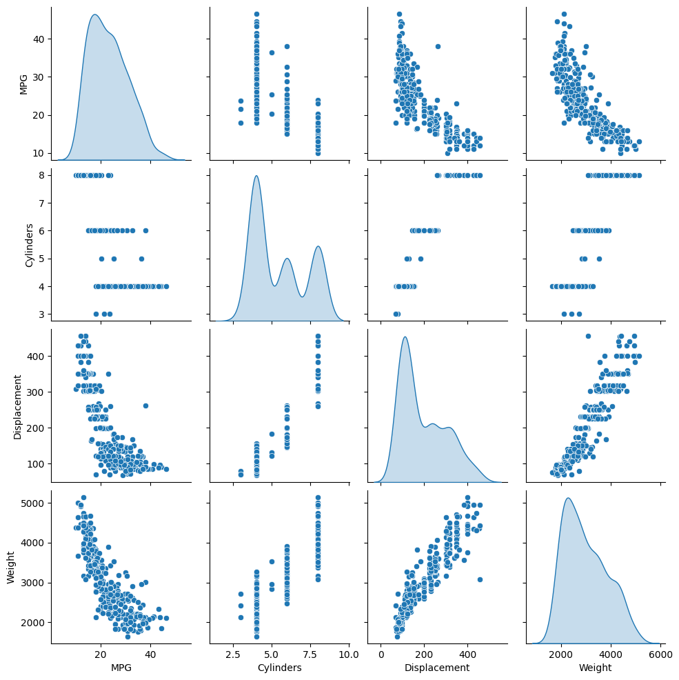
Review the joint distribution of a few pairs of columns from the training set.
The top row suggests that the fuel efficiency (MPG) is a function of all the other parameters. The other rows indicate they are functions of each other.
sns.pairplot(train_dataset[['MPG', 'Cylinders', 'Displacement', 'Weight']], diag_kind='kde')
<seaborn.axisgrid.PairGrid at 0x7f1b7f4ba160>
Let's also check the overall statistics. Note how each feature covers a very different range:
train_dataset.describe().transpose()
Split features from labels
Separate the target value—the "label"—from the features. This label is the value that you will train the model to predict.
train_features = train_dataset.copy()
test_features = test_dataset.copy()

train_labels = train_features.pop('MPG')
test_labels = test_features.pop('MPG')
Normalization
In the table of statistics it's easy to see how different the ranges of each feature are:
train_dataset.describe().transpose()[['mean', 'std']]
It is good practice to normalize features that use different scales and ranges.
One reason this is important is because the features are multiplied by the model weights. So, the scale of the outputs and the scale of the gradients are affected by the scale of the inputs.
Although a model might converge without feature normalization, normalization makes training much more stable.
The Normalization layer
The tf.keras.layers.Normalization is a clean and simple way to add feature normalization into your model.
The first step is to create the layer:
normalizer = tf.keras.layers.Normalization(axis=-1)
Then, fit the state of the preprocessing layer to the data by calling Normalization.adapt:
normalizer.adapt(np.array(train_features))
I0000 00:00:1764739589.952689  534406 gpu_device.cc:2019] Created device /job:localhost/replica:0/task:0/device:GPU:0 with 13638 MB memory:  -> device: 0, name: Tesla T4, pci bus id: 0000:00:05.0, compute capability: 7.5
I0000 00:00:1764739589.955003  534406 gpu_device.cc:2019] Created device /job:localhost/replica:0/task:0/device:GPU:1 with 13756 MB memory:  -> device: 1, name: Tesla T4, pci bus id: 0000:00:06.0, compute capability: 7.5
I0000 00:00:1764739589.957326  534406 gpu_device.cc:2019] Created device /job:localhost/replica:0/task:0/device:GPU:2 with 13756 MB memory:  -> device: 2, name: Tesla T4, pci bus id: 0000:00:07.0, compute capability: 7.5
I0000 00:00:1764739589.959535  534406 gpu_device.cc:2019] Created device /job:localhost/replica:0/task:0/device:GPU:3 with 13756 MB memory:  -> device: 3, name: Tesla T4, pci bus id: 0000:00:08.0, compute capability: 7.5
Calculate the mean and variance, and store them in the layer:
print(normalizer.mean.numpy())
[[   5.478  195.318  104.869 2990.252   15.559   75.898    0.178    0.197
     0.624]]
When the layer is called, it returns the input data, with each feature independently normalized:
first = np.array(train_features[:1])

with np.printoptions(precision=2, suppress=True):
  print('First example:', first)
  print()
  print('Normalized:', normalizer(first).numpy())
First example: [[   4.    90.    75.  2125.    14.5   74.     0.     0.     1. ]]
Normalized: [[-0.87 -1.01 -0.79 -1.03 -0.38 -0.52 -0.47 -0.5   0.78]]
Linear regression
Before building a deep neural network model, start with linear regression using one and several variables.
Linear regression with one variable
Begin with a single-variable linear regression to predict 'MPG' from 'Horsepower'.
Training a model with tf.keras typically starts by defining the model architecture. Use a tf.keras.Sequential model, which represents a sequence of steps.
There are two steps in your single-variable linear regression model:
- Normalize the
'Horsepower'input features using thetf.keras.layers.Normalizationpreprocessing layer. - Apply a linear transformation (\(y = mx+b\)) to produce 1 output using a linear layer (
tf.keras.layers.Dense).
The number of inputs can either be set by the input_shape argument, or automatically when the model is run for the first time.
First, create a NumPy array made of the 'Horsepower' features. Then, instantiate the tf.keras.layers.Normalization and fit its state to the horsepower data:
horsepower = np.array(train_features['Horsepower'])

horsepower_normalizer = layers.Normalization(input_shape=[1,], axis=None)
horsepower_normalizer.adapt(horsepower)
/tmpfs/src/tf_docs_env/lib/python3.9/site-packages/keras/src/layers/preprocessing/tf_data_layer.py:19: UserWarning: Do not pass an `input_shape`/`input_dim` argument to a layer. When using Sequential models, prefer using an `Input(shape)` object as the first layer in the model instead.
  super().__init__(**kwargs)
Build the Keras Sequential model:
horsepower_model = tf.keras.Sequential([
    horsepower_normalizer,
    layers.Dense(units=1)
])

horsepower_model.summary()
This model will predict 'MPG' from 'Horsepower'.
Run the untrained model on the first 10 'Horsepower' values. The output won't be good, but notice that it has the expected shape of (10, 1):
horsepower_model.predict(horsepower[:10])
1/1 ━━━━━━━━━━━━━━━━━━━━ 0s 238ms/step
WARNING: All log messages before absl::InitializeLog() is called are written to STDERR
I0000 00:00:1764739591.531101  534582 service.cc:152] XLA service 0x7f1960004ef0 initialized for platform CUDA (this does not guarantee that XLA will be used). Devices:
I0000 00:00:1764739591.531131  534582 service.cc:160]   StreamExecutor device (0): Tesla T4, Compute Capability 7.5
I0000 00:00:1764739591.531135  534582 service.cc:160]   StreamExecutor device (1): Tesla T4, Compute Capability 7.5
I0000 00:00:1764739591.531138  534582 service.cc:160]   StreamExecutor device (2): Tesla T4, Compute Capability 7.5
I0000 00:00:1764739591.531140  534582 service.cc:160]   StreamExecutor device (3): Tesla T4, Compute Capability 7.5
I0000 00:00:1764739591.561807  534582 cuda_dnn.cc:529] Loaded cuDNN version 91600
I0000 00:00:1764739591.654505  534582 device_compiler.h:188] Compiled cluster using XLA!  This line is logged at most once for the lifetime of the process.
array([[ 0.742],
       [ 0.419],
       [-1.37 ],
       [ 1.04 ],
       [ 0.941],
       [ 0.369],
       [ 1.115],
       [ 0.941],
       [ 0.245],
       [ 0.419]], dtype=float32)
Once the model is built, configure the training procedure using the Keras Model.compile method. The most important arguments to compile are the loss and the optimizer, since these define what will be optimized (mean_absolute_error) and how (using the tf.keras.optimizers.Adam).
horsepower_model.compile(
    optimizer=tf.keras.optimizers.Adam(learning_rate=0.1),
    loss='mean_absolute_error')
Use Keras Model.fit to execute the training for 100 epochs:
%%time
history = horsepower_model.fit(
    train_features['Horsepower'],
    train_labels,
    epochs=100,
    # Suppress logging.
    verbose=0,
    # Calculate validation results on 20% of the training data.
    validation_split = 0.2)
CPU times: user 11.4 s, sys: 11 s, total: 22.4 s
Wall time: 18.6 s
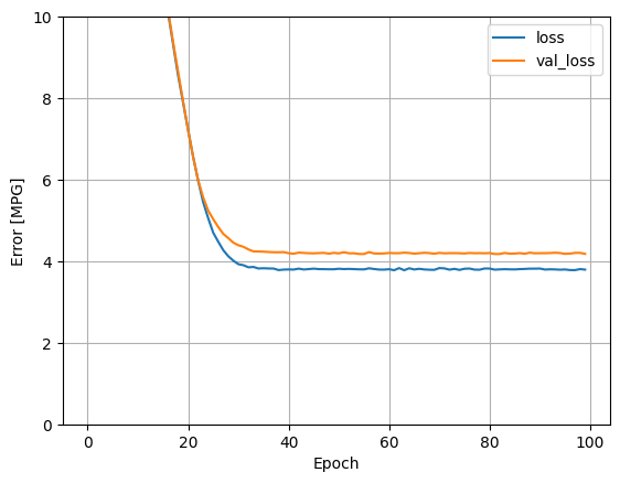
Visualize the model's training progress using the stats stored in the history object:
hist = pd.DataFrame(history.history)
hist['epoch'] = history.epoch
hist.tail()
def plot_loss(history):
  plt.plot(history.history['loss'], label='loss')
  plt.plot(history.history['val_loss'], label='val_loss')
  plt.ylim([0, 10])
  plt.xlabel('Epoch')
  plt.ylabel('Error [MPG]')
  plt.legend()
  plt.grid(True)
plot_loss(history)
Collect the results on the test set for later:
test_results = {}

test_results['horsepower_model'] = horsepower_model.evaluate(
    test_features['Horsepower'],
    test_labels, verbose=0)
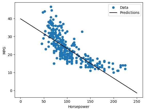
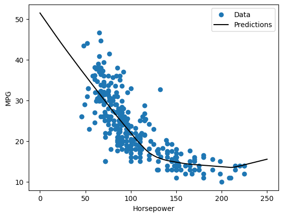
Since this is a single variable regression, it's easy to view the model's predictions as a function of the input:
x = tf.linspace(0.0, 250, 251)
y = horsepower_model.predict(x)
8/8 ━━━━━━━━━━━━━━━━━━━━ 0s 25ms/step
def plot_horsepower(x, y):
  plt.scatter(train_features['Horsepower'], train_labels, label='Data')
  plt.plot(x, y, color='k', label='Predictions')
  plt.xlabel('Horsepower')
  plt.ylabel('MPG')
  plt.legend()
plot_horsepower(x, y)
Linear regression with multiple inputs
You can use an almost identical setup to make predictions based on multiple inputs. This model still does the same \(y = mx+b\) except that \(m\) is a matrix and \(x\) is a vector.
Create a two-step Keras Sequential model again with the first layer being normalizer (tf.keras.layers.Normalization(axis=-1)) you defined earlier and adapted to the whole dataset:
linear_model = tf.keras.Sequential([
    normalizer,
    layers.Dense(units=1)
])
When you call Model.predict on a batch of inputs, it produces units=1 outputs for each example:
linear_model.predict(train_features[:10])
1/1 ━━━━━━━━━━━━━━━━━━━━ 0s 284ms/step
array([[ 0.767],
       [ 0.209],
       [ 2.26 ],
       [-0.651],
       [-2.402],
       [ 0.046],
       [-2.674],
       [-2.318],
       [ 0.796],
       [-1.165]], dtype=float32)
When you call the model, its weight matrices will be built—check that the kernel weights (the \(m\) in \(y=mx+b\)) have a shape of (9, 1):
linear_model.layers[1].kernel
<Variable path=sequential_1/dense_1/kernel, shape=(9, 1), dtype=float32, value=[[-0.343]
 [-0.238]
 [ 0.229]
 [ 0.699]
 [-0.352]
 [-0.59 ]
 [-0.712]
 [-0.645]
 [ 0.046]]>
Configure the model with Keras Model.compile and train with Model.fit for 100 epochs:
linear_model.compile(
    optimizer=tf.keras.optimizers.Adam(learning_rate=0.1),
    loss='mean_absolute_error')
%%time
history = linear_model.fit(
    train_features,
    train_labels,
    epochs=100,
    # Suppress logging.
    verbose=0,
    # Calculate validation results on 20% of the training data.
    validation_split = 0.2)
CPU times: user 11.5 s, sys: 11 s, total: 22.5 s
Wall time: 18.7 s
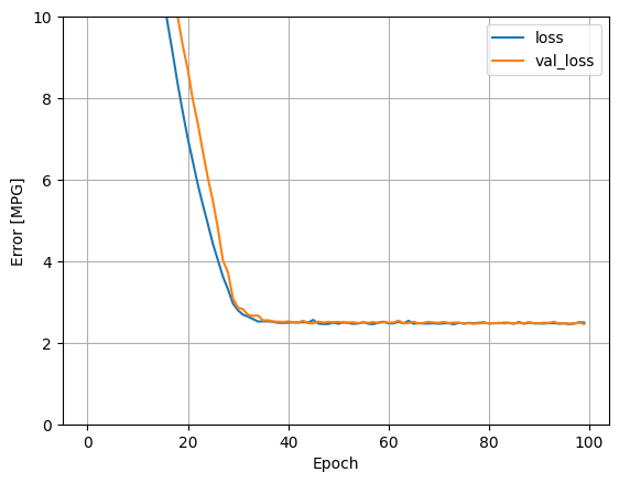
Using all the inputs in this regression model achieves a much lower training and validation error than the horsepower_model, which had one input:
plot_loss(history)
Collect the results on the test set for later:
test_results['linear_model'] = linear_model.evaluate(
    test_features, test_labels, verbose=0)
Regression with a deep neural network (DNN)
In the previous section, you implemented two linear models for single and multiple inputs.
Here, you will implement single-input and multiple-input DNN models.
The code is basically the same except the model is expanded to include some "hidden" non-linear layers. The name "hidden" here just means not directly connected to the inputs or outputs.
These models will contain a few more layers than the linear model:
- The normalization layer, as before (with
horsepower_normalizerfor a single-input model andnormalizerfor a multiple-input model). - Two hidden, non-linear,
Denselayers with the ReLU (relu) activation function nonlinearity. - A linear
Densesingle-output layer.
Both models will use the same training procedure, so the compile method is included in the build_and_compile_model function below.
def build_and_compile_model(norm):
  model = keras.Sequential([
      norm,
      layers.Dense(64, activation='relu'),
      layers.Dense(64, activation='relu'),
      layers.Dense(1)
  ])

  model.compile(loss='mean_absolute_error',
                optimizer=tf.keras.optimizers.Adam(0.001))
  return model
Regression using a DNN and a single input
Create a DNN model with only 'Horsepower' as input and horsepower_normalizer (defined earlier) as the normalization layer:
dnn_horsepower_model = build_and_compile_model(horsepower_normalizer)
This model has quite a few more trainable parameters than the linear models:
dnn_horsepower_model.summary()
Train the model with Keras Model.fit:
%%time
history = dnn_horsepower_model.fit(
    train_features['Horsepower'],
    train_labels,
    validation_split=0.2,
    verbose=0, epochs=100)
CPU times: user 12.5 s, sys: 11 s, total: 23.6 s
Wall time: 19.7 s
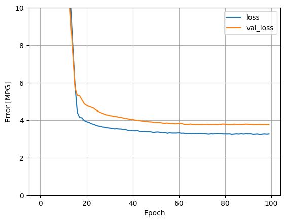
This model does slightly better than the linear single-input horsepower_model:
plot_loss(history)
If you plot the predictions as a function of 'Horsepower', you should notice how this model takes advantage of the nonlinearity provided by the hidden layers:
x = tf.linspace(0.0, 250, 251)
y = dnn_horsepower_model.predict(x)
WARNING:tensorflow:5 out of the last 11 calls to <function TensorFlowTrainer.make_predict_function.<locals>.one_step_on_data_distributed at 0x7f1acc0350d0> triggered tf.function retracing. Tracing is expensive and the excessive number of tracings could be due to (1) creating @tf.function repeatedly in a loop, (2) passing tensors with different shapes, (3) passing Python objects instead of tensors. For (1), please define your @tf.function outside of the loop. For (2), @tf.function has reduce_retracing=True option that can avoid unnecessary retracing. For (3), please refer to https://www.tensorflow.org/guide/function#controlling_retracing and https://www.tensorflow.org/api_docs/python/tf/function for  more details.
1/8 ━━━━━━━━━━━━━━━━━━━━ 1s 214ms/step
WARNING:tensorflow:5 out of the last 17 calls to <function TensorFlowTrainer.make_predict_function.<locals>.one_step_on_data_distributed at 0x7f1acc0350d0> triggered tf.function retracing. Tracing is expensive and the excessive number of tracings could be due to (1) creating @tf.function repeatedly in a loop, (2) passing tensors with different shapes, (3) passing Python objects instead of tensors. For (1), please define your @tf.function outside of the loop. For (2), @tf.function has reduce_retracing=True option that can avoid unnecessary retracing. For (3), please refer to https://www.tensorflow.org/guide/function#controlling_retracing and https://www.tensorflow.org/api_docs/python/tf/function for  more details.
8/8 ━━━━━━━━━━━━━━━━━━━━ 0s 32ms/step
plot_horsepower(x, y)
Collect the results on the test set for later:
test_results['dnn_horsepower_model'] = dnn_horsepower_model.evaluate(
    test_features['Horsepower'], test_labels,
    verbose=0)
Regression using a DNN and multiple inputs
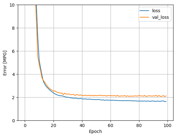
Repeat the previous process using all the inputs. The model's performance slightly improves on the validation dataset.
dnn_model = build_and_compile_model(normalizer)
dnn_model.summary()
%%time
history = dnn_model.fit(
    train_features,
    train_labels,
    validation_split=0.2,
    verbose=0, epochs=100)
CPU times: user 12.5 s, sys: 11.2 s, total: 23.7 s
Wall time: 19.8 s
plot_loss(history)
Collect the results on the test set:
test_results['dnn_model'] = dnn_model.evaluate(test_features, test_labels, verbose=0)
Performance
Since all models have been trained, you can review their test set performance:
pd.DataFrame(test_results, index=['Mean absolute error [MPG]']).T
These results match the validation error observed during training.
Make predictions
You can now make predictions with the dnn_model on the test set using Keras Model.predict and review the loss:
test_predictions = dnn_model.predict(test_features).flatten()

a = plt.axes(aspect='equal')
plt.scatter(test_labels, test_predictions)
plt.xlabel('True Values [MPG]')
plt.ylabel('Predictions [MPG]')
lims = [0, 50]
plt.xlim(lims)
plt.ylim(lims)
_ = plt.plot(lims, lims)
3/3 ━━━━━━━━━━━━━━━━━━━━ 0s 112ms/step
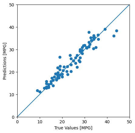
It appears that the model predicts reasonably well.
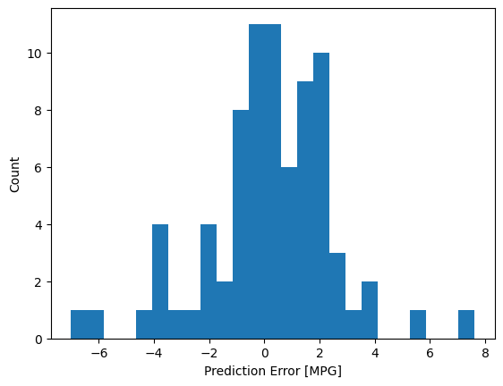
Now, check the error distribution:
error = test_predictions - test_labels
plt.hist(error, bins=25)
plt.xlabel('Prediction Error [MPG]')
_ = plt.ylabel('Count')
If you're happy with the model, save it for later use with Model.save:
dnn_model.save('dnn_model.keras')
If you reload the model, it gives identical output:
reloaded = tf.keras.models.load_model('dnn_model.keras')

test_results['reloaded'] = reloaded.evaluate(
    test_features, test_labels, verbose=0)
pd.DataFrame(test_results, index=['Mean absolute error [MPG]']).T
Conclusion
This notebook introduced a few techniques to handle a regression problem. Here are a few more tips that may help:
- Mean squared error (MSE) (
tf.keras.losses.MeanSquaredError) and mean absolute error (MAE) (tf.keras.losses.MeanAbsoluteError) are common loss functions used for regression problems. MAE is less sensitive to outliers. Different loss functions are used for classification problems. - Similarly, evaluation metrics used for regression differ from classification.
- When numeric input data features have values with different ranges, each feature should be scaled independently to the same range.
- Overfitting is a common problem for DNN models, though it wasn't a problem for this tutorial. Visit the Overfit and underfit tutorial for more help with this.
# MIT License
#
# Copyright (c) 2017 François Chollet
#
# Permission is hereby granted, free of charge, to any person obtaining a
# copy of this software and associated documentation files (the "Software"),
# to deal in the Software without restriction, including without limitation
# the rights to use, copy, modify, merge, publish, distribute, sublicense,
# and/or sell copies of the Software, and to permit persons to whom the
# Software is furnished to do so, subject to the following conditions:
#
# The above copyright notice and this permission notice shall be included in
# all copies or substantial portions of the Software.
#
# THE SOFTWARE IS PROVIDED "AS IS", WITHOUT WARRANTY OF ANY KIND, EXPRESS OR
# IMPLIED, INCLUDING BUT NOT LIMITED TO THE WARRANTIES OF MERCHANTABILITY,
# FITNESS FOR A PARTICULAR PURPOSE AND NONINFRINGEMENT. IN NO EVENT SHALL
# THE AUTHORS OR COPYRIGHT HOLDERS BE LIABLE FOR ANY CLAIM, DAMAGES OR OTHER
# LIABILITY, WHETHER IN AN ACTION OF CONTRACT, TORT OR OTHERWISE, ARISING
# FROM, OUT OF OR IN CONNECTION WITH THE SOFTWARE OR THE USE OR OTHER
# DEALINGS IN THE SOFTWARE.