
|
|
|
 View source on GitHub View source on GitHub
|
|
This guide trains a neural network model to classify images of clothing, like sneakers and shirts. It's okay if you don't understand all the details; this is a fast-paced overview of a complete TensorFlow program with the details explained as you go.
This guide uses tf.keras, a high-level API to build and train models in TensorFlow.
# TensorFlow and tf.keras
import tensorflow as tf

# Helper libraries
import numpy as np
import matplotlib.pyplot as plt

print(tf.__version__)
2024-08-16 01:20:39.960631: E external/local_xla/xla/stream_executor/cuda/cuda_fft.cc:485] Unable to register cuFFT factory: Attempting to register factory for plugin cuFFT when one has already been registered
2024-08-16 01:20:39.982110: E external/local_xla/xla/stream_executor/cuda/cuda_dnn.cc:8454] Unable to register cuDNN factory: Attempting to register factory for plugin cuDNN when one has already been registered
2024-08-16 01:20:39.988691: E external/local_xla/xla/stream_executor/cuda/cuda_blas.cc:1452] Unable to register cuBLAS factory: Attempting to register factory for plugin cuBLAS when one has already been registered
2.17.0
Import the Fashion MNIST dataset
This guide uses the Fashion MNIST dataset which contains 70,000 grayscale images in 10 categories. The images show individual articles of clothing at low resolution (28 by 28 pixels), as seen here:
|
|
|
Figure 1. Fashion-MNIST samples (by Zalando, MIT License). |
Fashion MNIST is intended as a drop-in replacement for the classic MNIST dataset—often used as the "Hello, World" of machine learning programs for computer vision. The MNIST dataset contains images of handwritten digits (0, 1, 2, etc.) in a format identical to that of the articles of clothing you'll use here.
This guide uses Fashion MNIST for variety, and because it's a slightly more challenging problem than regular MNIST. Both datasets are relatively small and are used to verify that an algorithm works as expected. They're good starting points to test and debug code.
Here, 60,000 images are used to train the network and 10,000 images to evaluate how accurately the network learned to classify images. You can access the Fashion MNIST directly from TensorFlow. Import and load the Fashion MNIST data directly from TensorFlow:
fashion_mnist = tf.keras.datasets.fashion_mnist

(train_images, train_labels), (test_images, test_labels) = fashion_mnist.load_data()
Downloading data from https://storage.googleapis.com/tensorflow/tf-keras-datasets/train-labels-idx1-ubyte.gz
29515/29515 ━━━━━━━━━━━━━━━━━━━━ 0s 0us/step
Downloading data from https://storage.googleapis.com/tensorflow/tf-keras-datasets/train-images-idx3-ubyte.gz
26421880/26421880 ━━━━━━━━━━━━━━━━━━━━ 0s 0us/step
Downloading data from https://storage.googleapis.com/tensorflow/tf-keras-datasets/t10k-labels-idx1-ubyte.gz
5148/5148 ━━━━━━━━━━━━━━━━━━━━ 0s 0us/step
Downloading data from https://storage.googleapis.com/tensorflow/tf-keras-datasets/t10k-images-idx3-ubyte.gz
4422102/4422102 ━━━━━━━━━━━━━━━━━━━━ 0s 0us/step
Loading the dataset returns four NumPy arrays:
- The
train_imagesandtrain_labelsarrays are the training set—the data the model uses to learn. - The model is tested against the test set, the
test_images, andtest_labelsarrays.
The images are 28x28 NumPy arrays, with pixel values ranging from 0 to 255. The labels are an array of integers, ranging from 0 to 9. These correspond to the class of clothing the image represents:
| Label | Class |
|---|---|
| 0 | T-shirt/top |
| 1 | Trouser |
| 2 | Pullover |
| 3 | Dress |
| 4 | Coat |
| 5 | Sandal |
| 6 | Shirt |
| 7 | Sneaker |
| 8 | Bag |
| 9 | Ankle boot |
Each image is mapped to a single label. Since the class names are not included with the dataset, store them here to use later when plotting the images:
class_names = ['T-shirt/top', 'Trouser', 'Pullover', 'Dress', 'Coat',
               'Sandal', 'Shirt', 'Sneaker', 'Bag', 'Ankle boot']
Explore the data
Let's explore the format of the dataset before training the model. The following shows there are 60,000 images in the training set, with each image represented as 28 x 28 pixels:
train_images.shape
(60000, 28, 28)
Likewise, there are 60,000 labels in the training set:
len(train_labels)
60000
Each label is an integer between 0 and 9:
train_labels
array([9, 0, 0, ..., 3, 0, 5], dtype=uint8)
There are 10,000 images in the test set. Again, each image is represented as 28 x 28 pixels:
test_images.shape
(10000, 28, 28)
And the test set contains 10,000 images labels:
len(test_labels)
10000
Preprocess the data
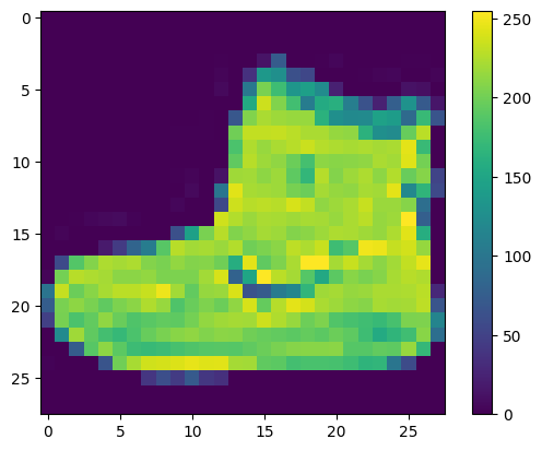
The data must be preprocessed before training the network. If you inspect the first image in the training set, you will see that the pixel values fall in the range of 0 to 255:
plt.figure()
plt.imshow(train_images[0])
plt.colorbar()
plt.grid(False)
plt.show()
Scale these values to a range of 0 to 1 before feeding them to the neural network model. To do so, divide the values by 255. It's important that the training set and the testing set be preprocessed in the same way:
train_images = train_images / 255.0

test_images = test_images / 255.0
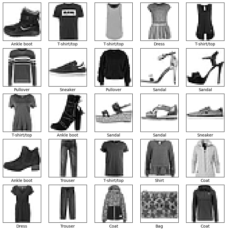
To verify that the data is in the correct format and that you're ready to build and train the network, let's display the first 25 images from the training set and display the class name below each image.
plt.figure(figsize=(10,10))
for i in range(25):
    plt.subplot(5,5,i+1)
    plt.xticks([])
    plt.yticks([])
    plt.grid(False)
    plt.imshow(train_images[i], cmap=plt.cm.binary)
    plt.xlabel(class_names[train_labels[i]])
plt.show()
Build the model
Building the neural network requires configuring the layers of the model, then compiling the model.
Set up the layers
The basic building block of a neural network is the layer. Layers extract representations from the data fed into them. Hopefully, these representations are meaningful for the problem at hand.
Most of deep learning consists of chaining together simple layers. Most layers, such as tf.keras.layers.Dense, have parameters that are learned during training.
model = tf.keras.Sequential([
    tf.keras.layers.Flatten(input_shape=(28, 28)),
    tf.keras.layers.Dense(128, activation='relu'),
    tf.keras.layers.Dense(10)
])
/tmpfs/src/tf_docs_env/lib/python3.9/site-packages/keras/src/layers/reshaping/flatten.py:37: UserWarning: Do not pass an `input_shape`/`input_dim` argument to a layer. When using Sequential models, prefer using an `Input(shape)` object as the first layer in the model instead.
  super().__init__(**kwargs)
WARNING: All log messages before absl::InitializeLog() is called are written to STDERR
I0000 00:00:1723771245.399945    8232 cuda_executor.cc:1015] successful NUMA node read from SysFS had negative value (-1), but there must be at least one NUMA node, so returning NUMA node zero. See more at https://github.com/torvalds/linux/blob/v6.0/Documentation/ABI/testing/sysfs-bus-pci#L344-L355
I0000 00:00:1723771245.403709    8232 cuda_executor.cc:1015] successful NUMA node read from SysFS had negative value (-1), but there must be at least one NUMA node, so returning NUMA node zero. See more at https://github.com/torvalds/linux/blob/v6.0/Documentation/ABI/testing/sysfs-bus-pci#L344-L355
I0000 00:00:1723771245.407479    8232 cuda_executor.cc:1015] successful NUMA node read from SysFS had negative value (-1), but there must be at least one NUMA node, so returning NUMA node zero. See more at https://github.com/torvalds/linux/blob/v6.0/Documentation/ABI/testing/sysfs-bus-pci#L344-L355
I0000 00:00:1723771245.411239    8232 cuda_executor.cc:1015] successful NUMA node read from SysFS had negative value (-1), but there must be at least one NUMA node, so returning NUMA node zero. See more at https://github.com/torvalds/linux/blob/v6.0/Documentation/ABI/testing/sysfs-bus-pci#L344-L355
I0000 00:00:1723771245.422243    8232 cuda_executor.cc:1015] successful NUMA node read from SysFS had negative value (-1), but there must be at least one NUMA node, so returning NUMA node zero. See more at https://github.com/torvalds/linux/blob/v6.0/Documentation/ABI/testing/sysfs-bus-pci#L344-L355
I0000 00:00:1723771245.425820    8232 cuda_executor.cc:1015] successful NUMA node read from SysFS had negative value (-1), but there must be at least one NUMA node, so returning NUMA node zero. See more at https://github.com/torvalds/linux/blob/v6.0/Documentation/ABI/testing/sysfs-bus-pci#L344-L355
I0000 00:00:1723771245.429273    8232 cuda_executor.cc:1015] successful NUMA node read from SysFS had negative value (-1), but there must be at least one NUMA node, so returning NUMA node zero. See more at https://github.com/torvalds/linux/blob/v6.0/Documentation/ABI/testing/sysfs-bus-pci#L344-L355
I0000 00:00:1723771245.432759    8232 cuda_executor.cc:1015] successful NUMA node read from SysFS had negative value (-1), but there must be at least one NUMA node, so returning NUMA node zero. See more at https://github.com/torvalds/linux/blob/v6.0/Documentation/ABI/testing/sysfs-bus-pci#L344-L355
I0000 00:00:1723771245.436119    8232 cuda_executor.cc:1015] successful NUMA node read from SysFS had negative value (-1), but there must be at least one NUMA node, so returning NUMA node zero. See more at https://github.com/torvalds/linux/blob/v6.0/Documentation/ABI/testing/sysfs-bus-pci#L344-L355
I0000 00:00:1723771245.439570    8232 cuda_executor.cc:1015] successful NUMA node read from SysFS had negative value (-1), but there must be at least one NUMA node, so returning NUMA node zero. See more at https://github.com/torvalds/linux/blob/v6.0/Documentation/ABI/testing/sysfs-bus-pci#L344-L355
I0000 00:00:1723771245.443002    8232 cuda_executor.cc:1015] successful NUMA node read from SysFS had negative value (-1), but there must be at least one NUMA node, so returning NUMA node zero. See more at https://github.com/torvalds/linux/blob/v6.0/Documentation/ABI/testing/sysfs-bus-pci#L344-L355
I0000 00:00:1723771245.446467    8232 cuda_executor.cc:1015] successful NUMA node read from SysFS had negative value (-1), but there must be at least one NUMA node, so returning NUMA node zero. See more at https://github.com/torvalds/linux/blob/v6.0/Documentation/ABI/testing/sysfs-bus-pci#L344-L355
I0000 00:00:1723771246.712159    8232 cuda_executor.cc:1015] successful NUMA node read from SysFS had negative value (-1), but there must be at least one NUMA node, so returning NUMA node zero. See more at https://github.com/torvalds/linux/blob/v6.0/Documentation/ABI/testing/sysfs-bus-pci#L344-L355
I0000 00:00:1723771246.714268    8232 cuda_executor.cc:1015] successful NUMA node read from SysFS had negative value (-1), but there must be at least one NUMA node, so returning NUMA node zero. See more at https://github.com/torvalds/linux/blob/v6.0/Documentation/ABI/testing/sysfs-bus-pci#L344-L355
I0000 00:00:1723771246.716341    8232 cuda_executor.cc:1015] successful NUMA node read from SysFS had negative value (-1), but there must be at least one NUMA node, so returning NUMA node zero. See more at https://github.com/torvalds/linux/blob/v6.0/Documentation/ABI/testing/sysfs-bus-pci#L344-L355
I0000 00:00:1723771246.718359    8232 cuda_executor.cc:1015] successful NUMA node read from SysFS had negative value (-1), but there must be at least one NUMA node, so returning NUMA node zero. See more at https://github.com/torvalds/linux/blob/v6.0/Documentation/ABI/testing/sysfs-bus-pci#L344-L355
I0000 00:00:1723771246.720355    8232 cuda_executor.cc:1015] successful NUMA node read from SysFS had negative value (-1), but there must be at least one NUMA node, so returning NUMA node zero. See more at https://github.com/torvalds/linux/blob/v6.0/Documentation/ABI/testing/sysfs-bus-pci#L344-L355
I0000 00:00:1723771246.722302    8232 cuda_executor.cc:1015] successful NUMA node read from SysFS had negative value (-1), but there must be at least one NUMA node, so returning NUMA node zero. See more at https://github.com/torvalds/linux/blob/v6.0/Documentation/ABI/testing/sysfs-bus-pci#L344-L355
I0000 00:00:1723771246.724257    8232 cuda_executor.cc:1015] successful NUMA node read from SysFS had negative value (-1), but there must be at least one NUMA node, so returning NUMA node zero. See more at https://github.com/torvalds/linux/blob/v6.0/Documentation/ABI/testing/sysfs-bus-pci#L344-L355
I0000 00:00:1723771246.726181    8232 cuda_executor.cc:1015] successful NUMA node read from SysFS had negative value (-1), but there must be at least one NUMA node, so returning NUMA node zero. See more at https://github.com/torvalds/linux/blob/v6.0/Documentation/ABI/testing/sysfs-bus-pci#L344-L355
I0000 00:00:1723771246.728090    8232 cuda_executor.cc:1015] successful NUMA node read from SysFS had negative value (-1), but there must be at least one NUMA node, so returning NUMA node zero. See more at https://github.com/torvalds/linux/blob/v6.0/Documentation/ABI/testing/sysfs-bus-pci#L344-L355
I0000 00:00:1723771246.730035    8232 cuda_executor.cc:1015] successful NUMA node read from SysFS had negative value (-1), but there must be at least one NUMA node, so returning NUMA node zero. See more at https://github.com/torvalds/linux/blob/v6.0/Documentation/ABI/testing/sysfs-bus-pci#L344-L355
I0000 00:00:1723771246.731978    8232 cuda_executor.cc:1015] successful NUMA node read from SysFS had negative value (-1), but there must be at least one NUMA node, so returning NUMA node zero. See more at https://github.com/torvalds/linux/blob/v6.0/Documentation/ABI/testing/sysfs-bus-pci#L344-L355
I0000 00:00:1723771246.733907    8232 cuda_executor.cc:1015] successful NUMA node read from SysFS had negative value (-1), but there must be at least one NUMA node, so returning NUMA node zero. See more at https://github.com/torvalds/linux/blob/v6.0/Documentation/ABI/testing/sysfs-bus-pci#L344-L355
I0000 00:00:1723771246.773205    8232 cuda_executor.cc:1015] successful NUMA node read from SysFS had negative value (-1), but there must be at least one NUMA node, so returning NUMA node zero. See more at https://github.com/torvalds/linux/blob/v6.0/Documentation/ABI/testing/sysfs-bus-pci#L344-L355
I0000 00:00:1723771246.775242    8232 cuda_executor.cc:1015] successful NUMA node read from SysFS had negative value (-1), but there must be at least one NUMA node, so returning NUMA node zero. See more at https://github.com/torvalds/linux/blob/v6.0/Documentation/ABI/testing/sysfs-bus-pci#L344-L355
I0000 00:00:1723771246.777277    8232 cuda_executor.cc:1015] successful NUMA node read from SysFS had negative value (-1), but there must be at least one NUMA node, so returning NUMA node zero. See more at https://github.com/torvalds/linux/blob/v6.0/Documentation/ABI/testing/sysfs-bus-pci#L344-L355
I0000 00:00:1723771246.779277    8232 cuda_executor.cc:1015] successful NUMA node read from SysFS had negative value (-1), but there must be at least one NUMA node, so returning NUMA node zero. See more at https://github.com/torvalds/linux/blob/v6.0/Documentation/ABI/testing/sysfs-bus-pci#L344-L355
I0000 00:00:1723771246.781323    8232 cuda_executor.cc:1015] successful NUMA node read from SysFS had negative value (-1), but there must be at least one NUMA node, so returning NUMA node zero. See more at https://github.com/torvalds/linux/blob/v6.0/Documentation/ABI/testing/sysfs-bus-pci#L344-L355
I0000 00:00:1723771246.783269    8232 cuda_executor.cc:1015] successful NUMA node read from SysFS had negative value (-1), but there must be at least one NUMA node, so returning NUMA node zero. See more at https://github.com/torvalds/linux/blob/v6.0/Documentation/ABI/testing/sysfs-bus-pci#L344-L355
I0000 00:00:1723771246.785254    8232 cuda_executor.cc:1015] successful NUMA node read from SysFS had negative value (-1), but there must be at least one NUMA node, so returning NUMA node zero. See more at https://github.com/torvalds/linux/blob/v6.0/Documentation/ABI/testing/sysfs-bus-pci#L344-L355
I0000 00:00:1723771246.787201    8232 cuda_executor.cc:1015] successful NUMA node read from SysFS had negative value (-1), but there must be at least one NUMA node, so returning NUMA node zero. See more at https://github.com/torvalds/linux/blob/v6.0/Documentation/ABI/testing/sysfs-bus-pci#L344-L355
I0000 00:00:1723771246.789148    8232 cuda_executor.cc:1015] successful NUMA node read from SysFS had negative value (-1), but there must be at least one NUMA node, so returning NUMA node zero. See more at https://github.com/torvalds/linux/blob/v6.0/Documentation/ABI/testing/sysfs-bus-pci#L344-L355
I0000 00:00:1723771246.792670    8232 cuda_executor.cc:1015] successful NUMA node read from SysFS had negative value (-1), but there must be at least one NUMA node, so returning NUMA node zero. See more at https://github.com/torvalds/linux/blob/v6.0/Documentation/ABI/testing/sysfs-bus-pci#L344-L355
I0000 00:00:1723771246.795758    8232 cuda_executor.cc:1015] successful NUMA node read from SysFS had negative value (-1), but there must be at least one NUMA node, so returning NUMA node zero. See more at https://github.com/torvalds/linux/blob/v6.0/Documentation/ABI/testing/sysfs-bus-pci#L344-L355
I0000 00:00:1723771246.798118    8232 cuda_executor.cc:1015] successful NUMA node read from SysFS had negative value (-1), but there must be at least one NUMA node, so returning NUMA node zero. See more at https://github.com/torvalds/linux/blob/v6.0/Documentation/ABI/testing/sysfs-bus-pci#L344-L355
The first layer in this network, tf.keras.layers.Flatten, transforms the format of the images from a two-dimensional array (of 28 by 28 pixels) to a one-dimensional array (of 28 * 28 = 784 pixels). Think of this layer as unstacking rows of pixels in the image and lining them up. This layer has no parameters to learn; it only reformats the data.
After the pixels are flattened, the network consists of a sequence of two tf.keras.layers.Dense layers. These are densely connected, or fully connected, neural layers. The first Dense layer has 128 nodes (or neurons). The second (and last) layer returns a logits array with length of 10. Each node contains a score that indicates the current image belongs to one of the 10 classes.
Compile the model
Before the model is ready for training, it needs a few more settings. These are added during the model's compile step:
- Optimizer —This is how the model is updated based on the data it sees and its loss function.
- Loss function —This measures how accurate the model is during training. You want to minimize this function to "steer" the model in the right direction.
- Metrics —Used to monitor the training and testing steps. The following example uses accuracy, the fraction of the images that are correctly classified.
model.compile(optimizer='adam',
              loss=tf.keras.losses.SparseCategoricalCrossentropy(from_logits=True),
              metrics=['accuracy'])
Train the model
Training the neural network model requires the following steps:
- Feed the training data to the model. In this example, the training data is in the
train_imagesandtrain_labelsarrays. - The model learns to associate images and labels.
- You ask the model to make predictions about a test set—in this example, the
test_imagesarray. - Verify that the predictions match the labels from the
test_labelsarray.
Feed the model
To start training, call the model.fit method—so called because it "fits" the model to the training data:
model.fit(train_images, train_labels, epochs=10)
Epoch 1/10
WARNING: All log messages before absl::InitializeLog() is called are written to STDERR
I0000 00:00:1723771249.187940    8438 service.cc:146] XLA service 0x7f4a6c007630 initialized for platform CUDA (this does not guarantee that XLA will be used). Devices:
I0000 00:00:1723771249.187968    8438 service.cc:154]   StreamExecutor device (0): Tesla T4, Compute Capability 7.5
I0000 00:00:1723771249.187973    8438 service.cc:154]   StreamExecutor device (1): Tesla T4, Compute Capability 7.5
I0000 00:00:1723771249.187976    8438 service.cc:154]   StreamExecutor device (2): Tesla T4, Compute Capability 7.5
I0000 00:00:1723771249.187979    8438 service.cc:154]   StreamExecutor device (3): Tesla T4, Compute Capability 7.5
125/1875 ━━━━━━━━━━━━━━━━━━━━ 2s 1ms/step - accuracy: 0.5742 - loss: 1.2336
I0000 00:00:1723771250.049424    8438 device_compiler.h:188] Compiled cluster using XLA!  This line is logged at most once for the lifetime of the process.
1875/1875 ━━━━━━━━━━━━━━━━━━━━ 4s 1ms/step - accuracy: 0.7842 - loss: 0.6205
Epoch 2/10
1875/1875 ━━━━━━━━━━━━━━━━━━━━ 2s 1ms/step - accuracy: 0.8607 - loss: 0.3859
Epoch 3/10
1875/1875 ━━━━━━━━━━━━━━━━━━━━ 2s 1ms/step - accuracy: 0.8768 - loss: 0.3384
Epoch 4/10
1875/1875 ━━━━━━━━━━━━━━━━━━━━ 2s 1ms/step - accuracy: 0.8842 - loss: 0.3138
Epoch 5/10
1875/1875 ━━━━━━━━━━━━━━━━━━━━ 2s 1ms/step - accuracy: 0.8915 - loss: 0.2939
Epoch 6/10
1875/1875 ━━━━━━━━━━━━━━━━━━━━ 2s 1ms/step - accuracy: 0.8944 - loss: 0.2868
Epoch 7/10
1875/1875 ━━━━━━━━━━━━━━━━━━━━ 2s 1ms/step - accuracy: 0.8990 - loss: 0.2700
Epoch 8/10
1875/1875 ━━━━━━━━━━━━━━━━━━━━ 2s 1ms/step - accuracy: 0.9012 - loss: 0.2623
Epoch 9/10
1875/1875 ━━━━━━━━━━━━━━━━━━━━ 2s 1ms/step - accuracy: 0.9091 - loss: 0.2476
Epoch 10/10
1875/1875 ━━━━━━━━━━━━━━━━━━━━ 2s 1ms/step - accuracy: 0.9107 - loss: 0.2364
<keras.src.callbacks.history.History at 0x7f4d31649eb0>
As the model trains, the loss and accuracy metrics are displayed. This model reaches an accuracy of about 0.91 (or 91%) on the training data.
Evaluate accuracy
Next, compare how the model performs on the test dataset:
test_loss, test_acc = model.evaluate(test_images,  test_labels, verbose=2)

print('\nTest accuracy:', test_acc)
313/313 - 1s - 3ms/step - accuracy: 0.8863 - loss: 0.3257

Test accuracy: 0.8863000273704529
It turns out that the accuracy on the test dataset is a little less than the accuracy on the training dataset. This gap between training accuracy and test accuracy represents overfitting. Overfitting happens when a machine learning model performs worse on new, previously unseen inputs than it does on the training data. An overfitted model "memorizes" the noise and details in the training dataset to a point where it negatively impacts the performance of the model on the new data. For more information, see the following:
Make predictions
With the model trained, you can use it to make predictions about some images. Attach a softmax layer to convert the model's linear outputs—logits—to probabilities, which should be easier to interpret.
probability_model = tf.keras.Sequential([model,
                                         tf.keras.layers.Softmax()])
predictions = probability_model.predict(test_images)
313/313 ━━━━━━━━━━━━━━━━━━━━ 1s 1ms/step
Here, the model has predicted the label for each image in the testing set. Let's take a look at the first prediction:
predictions[0]
array([6.8082486e-06, 8.7130829e-08, 2.3059203e-08, 1.7164245e-08,
       9.2101942e-07, 1.5966746e-03, 3.3436372e-06, 1.1623867e-02,
       4.7985890e-07, 9.8676783e-01], dtype=float32)
A prediction is an array of 10 numbers. They represent the model's "confidence" that the image corresponds to each of the 10 different articles of clothing. You can see which label has the highest confidence value:
np.argmax(predictions[0])
9
So, the model is most confident that this image is an ankle boot, or class_names[9]. Examining the test label shows that this classification is correct:
test_labels[0]
9
Define functions to graph the full set of 10 class predictions.
def plot_image(i, predictions_array, true_label, img):
  true_label, img = true_label[i], img[i]
  plt.grid(False)
  plt.xticks([])
  plt.yticks([])

  plt.imshow(img, cmap=plt.cm.binary)

  predicted_label = np.argmax(predictions_array)
  if predicted_label == true_label:
    color = 'blue'
  else:
    color = 'red'

  plt.xlabel("{} {:2.0f}% ({})".format(class_names[predicted_label],
                                100*np.max(predictions_array),
                                class_names[true_label]),
                                color=color)

def plot_value_array(i, predictions_array, true_label):
  true_label = true_label[i]
  plt.grid(False)
  plt.xticks(range(10))
  plt.yticks([])
  thisplot = plt.bar(range(10), predictions_array, color="#777777")
  plt.ylim([0, 1])
  predicted_label = np.argmax(predictions_array)

  thisplot[predicted_label].set_color('red')
  thisplot[true_label].set_color('blue')
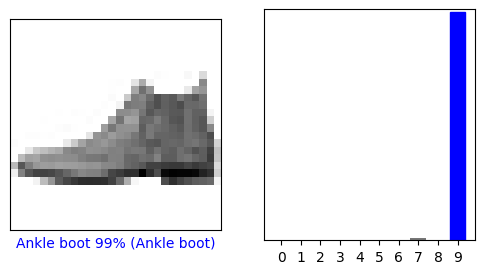
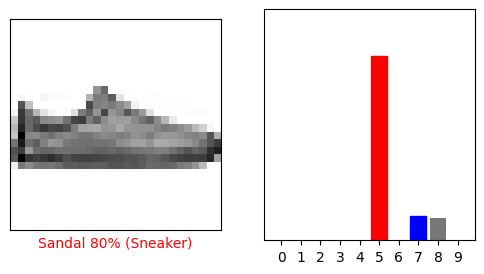
Verify predictions
With the model trained, you can use it to make predictions about some images.
Let's look at the 0th image, predictions, and prediction array. Correct prediction labels are blue and incorrect prediction labels are red. The number gives the percentage (out of 100) for the predicted label.
i = 0
plt.figure(figsize=(6,3))
plt.subplot(1,2,1)
plot_image(i, predictions[i], test_labels, test_images)
plt.subplot(1,2,2)
plot_value_array(i, predictions[i],  test_labels)
plt.show()
i = 12
plt.figure(figsize=(6,3))
plt.subplot(1,2,1)
plot_image(i, predictions[i], test_labels, test_images)
plt.subplot(1,2,2)
plot_value_array(i, predictions[i],  test_labels)
plt.show()
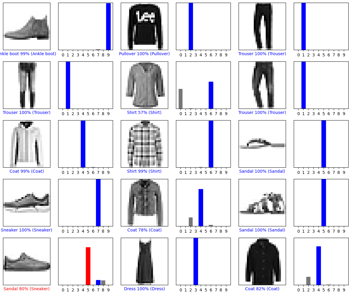
Let's plot several images with their predictions. Note that the model can be wrong even when very confident.
# Plot the first X test images, their predicted labels, and the true labels.
# Color correct predictions in blue and incorrect predictions in red.
num_rows = 5
num_cols = 3
num_images = num_rows*num_cols
plt.figure(figsize=(2*2*num_cols, 2*num_rows))
for i in range(num_images):
  plt.subplot(num_rows, 2*num_cols, 2*i+1)
  plot_image(i, predictions[i], test_labels, test_images)
  plt.subplot(num_rows, 2*num_cols, 2*i+2)
  plot_value_array(i, predictions[i], test_labels)
plt.tight_layout()
plt.show()
Use the trained model
Finally, use the trained model to make a prediction about a single image.
# Grab an image from the test dataset.
img = test_images[1]

print(img.shape)
(28, 28)
tf.keras models are optimized to make predictions on a batch, or collection, of examples at once. Accordingly, even though you're using a single image, you need to add it to a list:
# Add the image to a batch where it's the only member.
img = (np.expand_dims(img,0))

print(img.shape)
(1, 28, 28)
Now predict the correct label for this image:
predictions_single = probability_model.predict(img)

print(predictions_single)
1/1 ━━━━━━━━━━━━━━━━━━━━ 0s 146ms/step
[[4.0262650e-05 1.7603366e-12 9.9607229e-01 4.6822952e-11 3.8338848e-03
  1.7586101e-10 5.3584125e-05 7.4621548e-13 5.4244734e-12 5.0442324e-15]]
plot_value_array(1, predictions_single[0], test_labels)
_ = plt.xticks(range(10), class_names, rotation=45)
plt.show()
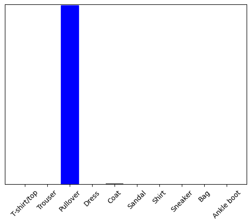
tf.keras.Model.predict returns a list of lists—one list for each image in the batch of data. Grab the predictions for our (only) image in the batch:
np.argmax(predictions_single[0])
2
And the model predicts a label as expected.
To learn more about building models with Keras, see the Keras guides.
# MIT License
#
# Copyright (c) 2017 François Chollet
#
# Permission is hereby granted, free of charge, to any person obtaining a
# copy of this software and associated documentation files (the "Software"),
# to deal in the Software without restriction, including without limitation
# the rights to use, copy, modify, merge, publish, distribute, sublicense,
# and/or sell copies of the Software, and to permit persons to whom the
# Software is furnished to do so, subject to the following conditions:
#
# The above copyright notice and this permission notice shall be included in
# all copies or substantial portions of the Software.
#
# THE SOFTWARE IS PROVIDED "AS IS", WITHOUT WARRANTY OF ANY KIND, EXPRESS OR
# IMPLIED, INCLUDING BUT NOT LIMITED TO THE WARRANTIES OF MERCHANTABILITY,
# FITNESS FOR A PARTICULAR PURPOSE AND NONINFRINGEMENT. IN NO EVENT SHALL
# THE AUTHORS OR COPYRIGHT HOLDERS BE LIABLE FOR ANY CLAIM, DAMAGES OR OTHER
# LIABILITY, WHETHER IN AN ACTION OF CONTRACT, TORT OR OTHERWISE, ARISING
# FROM, OUT OF OR IN CONNECTION WITH THE SOFTWARE OR THE USE OR OTHER
# DEALINGS IN THE SOFTWARE.