
| | |  ดูแหล่งที่มาบน GitHub ดูแหล่งที่มาบน GitHub | |
ภาพรวม
กวดวิชานี้จะแสดงให้เห็นถึงวิธีการที่ TensorFlow Lattice (TFL) ห้องสมุดสามารถนำมาใช้กับรุ่นรถไฟที่มีพฤติกรรมความรับผิดชอบและไม่ได้ละเมิดสมมติฐานบางอย่างที่มีจริยธรรมหรือยุติธรรม โดยเฉพาะอย่างยิ่งเราจะมุ่งเน้นการใช้ข้อ จำกัด monotonicity เพื่อหลีกเลี่ยงการลงโทษที่ไม่เป็นธรรมของคุณลักษณะบางอย่าง กวดวิชานี้จะรวมถึงการสาธิตการทดลองจากกระดาษ Deontological จริยธรรมโดย monotonicity จำกัด รูปร่าง โดยเซเรนาวังและยาแคนด์ตีพิมพ์ AISTATS 2020
เราจะใช้ตัวประมาณค่ากระป๋อง TFL กับชุดข้อมูลสาธารณะ แต่โปรดทราบว่าทุกอย่างในบทช่วยสอนนี้สามารถทำได้ด้วยแบบจำลองที่สร้างจากเลเยอร์ TFL Keras
ก่อนดำเนินการต่อ ตรวจสอบให้แน่ใจว่ารันไทม์ของคุณมีแพ็คเกจที่จำเป็นทั้งหมดติดตั้งอยู่ (ตามที่นำเข้ามาในเซลล์โค้ดด้านล่าง)
ติดตั้ง
การติดตั้งแพ็คเกจ TF Lattice:
pip install tensorflow-lattice seaborn
การนำเข้าแพ็คเกจที่จำเป็น:
import tensorflow as tf

import logging
import matplotlib.pyplot as plt
import numpy as np
import os
import pandas as pd
import seaborn as sns
from sklearn.model_selection import train_test_split
import sys
import tensorflow_lattice as tfl
logging.disable(sys.maxsize)
ค่าเริ่มต้นที่ใช้ในบทช่วยสอนนี้:
# List of learning rate hyperparameters to try.
# For a longer list of reasonable hyperparameters, try [0.001, 0.01, 0.1].
LEARNING_RATES = [0.01]
# Default number of training epochs and batch sizes.
NUM_EPOCHS = 1000
BATCH_SIZE = 1000
# Directory containing dataset files.
DATA_DIR = 'https://raw.githubusercontent.com/serenalwang/shape_constraints_for_ethics/master'
กรณีศึกษา #1: การรับเข้าเรียนในโรงเรียนกฎหมาย
ในส่วนแรกของบทช่วยสอนนี้ เราจะพิจารณากรณีศึกษาโดยใช้ชุดข้อมูล Law School Admissions จาก Law School Admissions Council (LSAC) เราจะฝึกตัวแยกประเภทเพื่อทำนายว่านักเรียนจะผ่านเกณฑ์หรือไม่โดยใช้สองคุณสมบัติ: คะแนน LSAT ของนักเรียนและเกรดเฉลี่ยในระดับปริญญาตรี
สมมติว่าคะแนนของลักษณนามถูกใช้เพื่อเป็นแนวทางในการเข้าศึกษาในโรงเรียนกฎหมายหรือทุนการศึกษา ตามบรรทัดฐานทางสังคมตามบุญ เราคาดหวังว่านักเรียนที่มีเกรดเฉลี่ยสูงกว่าและคะแนน LSAT สูงกว่าควรได้รับคะแนนที่สูงขึ้นจากตัวแยกประเภท อย่างไรก็ตาม เราจะสังเกตว่ามันง่ายสำหรับตัวแบบที่จะละเมิดบรรทัดฐานที่เข้าใจได้ง่ายเหล่านี้ และบางครั้งก็ลงโทษผู้ที่มีคะแนน GPA หรือ LSAT สูงกว่า
การแก้ไขปัญหาการปรับไหมนี้เป็นธรรมที่เราสามารถกำหนดข้อ จำกัด monotonicity เพื่อให้รูปแบบที่ไม่เคยลงโทษสูงกว่าเกรดเฉลี่ยหรือโหลดสูงกว่าคะแนน, สิ่งอื่นใดที่เท่าเทียมกัน ในบทช่วยสอนนี้ เราจะแสดงวิธีกำหนดข้อจำกัดความซ้ำซากจำเจโดยใช้ TFL
โหลดข้อมูลโรงเรียนกฎหมาย
# Load data file.
law_file_name = 'lsac.csv'
law_file_path = os.path.join(DATA_DIR, law_file_name)
raw_law_df = pd.read_csv(law_file_path, delimiter=',')
ชุดข้อมูลประมวลผลล่วงหน้า:
# Define label column name.
LAW_LABEL = 'pass_bar'
def preprocess_law_data(input_df):
  # Drop rows with where the label or features of interest are missing.
  output_df = input_df[~input_df[LAW_LABEL].isna() & ~input_df['ugpa'].isna() &
                       (input_df['ugpa'] > 0) & ~input_df['lsat'].isna()]
  return output_df


law_df = preprocess_law_data(raw_law_df)
แยกข้อมูลออกเป็นชุดฝึก/ตรวจสอบ/ทดสอบ
def split_dataset(input_df, random_state=888):
  """Splits an input dataset into train, val, and test sets."""
  train_df, test_val_df = train_test_split(
      input_df, test_size=0.3, random_state=random_state)
  val_df, test_df = train_test_split(
      test_val_df, test_size=0.66, random_state=random_state)
  return train_df, val_df, test_df


law_train_df, law_val_df, law_test_df = split_dataset(law_df)
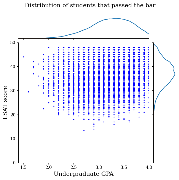
แสดงภาพการกระจายข้อมูล
ขั้นแรกเราจะเห็นภาพการกระจายของข้อมูล เราจะพล็อตคะแนน GPA และ LSAT สำหรับนักเรียนทุกคนที่ผ่านเกณฑ์และสำหรับนักเรียนทุกคนที่สอบไม่ผ่านเกณฑ์
def plot_dataset_contour(input_df, title):
  plt.rcParams['font.family'] = ['serif']
  g = sns.jointplot(
      x='ugpa',
      y='lsat',
      data=input_df,
      kind='kde',
      xlim=[1.4, 4],
      ylim=[0, 50])
  g.plot_joint(plt.scatter, c='b', s=10, linewidth=1, marker='+')
  g.ax_joint.collections[0].set_alpha(0)
  g.set_axis_labels('Undergraduate GPA', 'LSAT score', fontsize=14)
  g.fig.suptitle(title, fontsize=14)
  # Adust plot so that the title fits.
  plt.subplots_adjust(top=0.9)
  plt.show()
law_df_pos = law_df[law_df[LAW_LABEL] == 1]
plot_dataset_contour(
    law_df_pos, title='Distribution of students that passed the bar')
law_df_neg = law_df[law_df[LAW_LABEL] == 0]
plot_dataset_contour(
    law_df_neg, title='Distribution of students that failed the bar')

ฝึกปรับเทียบแบบจำลองเชิงเส้นเพื่อทำนายข้อสอบบาร์
ต่อไปเราจะฝึกรูปแบบเชิงเส้นการสอบเทียบจาก TFL ที่จะคาดการณ์หรือไม่ว่านักเรียนจะผ่านบาร์ คุณสมบัติการป้อนข้อมูลทั้งสองจะเป็นคะแนน LSAT และเกรดเฉลี่ยระดับปริญญาตรี และป้ายกำกับการฝึกอบรมจะเป็นว่านักเรียนผ่านบาร์หรือไม่
อันดับแรก เราจะฝึกโมเดลเชิงเส้นที่สอบเทียบโดยไม่มีข้อจำกัดใดๆ จากนั้น เราจะฝึกแบบจำลองเชิงเส้นตรงที่ปรับเทียบแล้วโดยมีข้อจำกัดความซ้ำซากจำเจ และสังเกตความแตกต่างในผลลัพธ์ของแบบจำลองและความแม่นยำ
ฟังก์ชันตัวช่วยสำหรับการฝึกอบรมตัวประมาณเชิงเส้นที่สอบเทียบ TFL
ฟังก์ชันเหล่านี้จะใช้สำหรับกรณีศึกษาของโรงเรียนกฎหมายนี้ เช่นเดียวกับกรณีศึกษาการผิดนัดชำระหนี้ด้านล่าง
def train_tfl_estimator(train_df, monotonicity, learning_rate, num_epochs,
                        batch_size, get_input_fn,
                        get_feature_columns_and_configs):
  """Trains a TFL calibrated linear estimator.

  Args:
    train_df: pandas dataframe containing training data.
    monotonicity: if 0, then no monotonicity constraints. If 1, then all
      features are constrained to be monotonically increasing.
    learning_rate: learning rate of Adam optimizer for gradient descent.
    num_epochs: number of training epochs.
    batch_size: batch size for each epoch. None means the batch size is the full
      dataset size.
    get_input_fn: function that returns the input_fn for a TF estimator.
    get_feature_columns_and_configs: function that returns TFL feature columns
      and configs.

  Returns:
    estimator: a trained TFL calibrated linear estimator.

  """
  feature_columns, feature_configs = get_feature_columns_and_configs(
      monotonicity)

  model_config = tfl.configs.CalibratedLinearConfig(
      feature_configs=feature_configs, use_bias=False)

  estimator = tfl.estimators.CannedClassifier(
      feature_columns=feature_columns,
      model_config=model_config,
      feature_analysis_input_fn=get_input_fn(input_df=train_df, num_epochs=1),
      optimizer=tf.keras.optimizers.Adam(learning_rate))

  estimator.train(
      input_fn=get_input_fn(
          input_df=train_df, num_epochs=num_epochs, batch_size=batch_size))
  return estimator


def optimize_learning_rates(
    train_df,
    val_df,
    test_df,
    monotonicity,
    learning_rates,
    num_epochs,
    batch_size,
    get_input_fn,
    get_feature_columns_and_configs,
):
  """Optimizes learning rates for TFL estimators.

  Args:
    train_df: pandas dataframe containing training data.
    val_df: pandas dataframe containing validation data.
    test_df: pandas dataframe containing test data.
    monotonicity: if 0, then no monotonicity constraints. If 1, then all
      features are constrained to be monotonically increasing.
    learning_rates: list of learning rates to try.
    num_epochs: number of training epochs.
    batch_size: batch size for each epoch. None means the batch size is the full
      dataset size.
    get_input_fn: function that returns the input_fn for a TF estimator.
    get_feature_columns_and_configs: function that returns TFL feature columns
      and configs.

  Returns:
    A single TFL estimator that achieved the best validation accuracy.
  """
  estimators = []
  train_accuracies = []
  val_accuracies = []
  test_accuracies = []
  for lr in learning_rates:
    estimator = train_tfl_estimator(
        train_df=train_df,
        monotonicity=monotonicity,
        learning_rate=lr,
        num_epochs=num_epochs,
        batch_size=batch_size,
        get_input_fn=get_input_fn,
        get_feature_columns_and_configs=get_feature_columns_and_configs)
    estimators.append(estimator)
    train_acc = estimator.evaluate(
        input_fn=get_input_fn(train_df, num_epochs=1))['accuracy']
    val_acc = estimator.evaluate(
        input_fn=get_input_fn(val_df, num_epochs=1))['accuracy']
    test_acc = estimator.evaluate(
        input_fn=get_input_fn(test_df, num_epochs=1))['accuracy']
    print('accuracies for learning rate %f: train: %f, val: %f, test: %f' %
          (lr, train_acc, val_acc, test_acc))
    train_accuracies.append(train_acc)
    val_accuracies.append(val_acc)
    test_accuracies.append(test_acc)
  max_index = val_accuracies.index(max(val_accuracies))
  return estimators[max_index]
ฟังก์ชันตัวช่วยสำหรับการกำหนดค่าคุณสมบัติชุดข้อมูลของโรงเรียนกฎหมาย
ฟังก์ชันตัวช่วยเหล่านี้เป็นกรณีศึกษาของโรงเรียนกฎหมายโดยเฉพาะ
def get_input_fn_law(input_df, num_epochs, batch_size=None):
  """Gets TF input_fn for law school models."""
  return tf.compat.v1.estimator.inputs.pandas_input_fn(
      x=input_df[['ugpa', 'lsat']],
      y=input_df['pass_bar'],
      num_epochs=num_epochs,
      batch_size=batch_size or len(input_df),
      shuffle=False)


def get_feature_columns_and_configs_law(monotonicity):
  """Gets TFL feature configs for law school models."""
  feature_columns = [
      tf.feature_column.numeric_column('ugpa'),
      tf.feature_column.numeric_column('lsat'),
  ]
  feature_configs = [
      tfl.configs.FeatureConfig(
          name='ugpa',
          lattice_size=2,
          pwl_calibration_num_keypoints=20,
          monotonicity=monotonicity,
          pwl_calibration_always_monotonic=False),
      tfl.configs.FeatureConfig(
          name='lsat',
          lattice_size=2,
          pwl_calibration_num_keypoints=20,
          monotonicity=monotonicity,
          pwl_calibration_always_monotonic=False),
  ]
  return feature_columns, feature_configs
ฟังก์ชันตัวช่วยสำหรับการแสดงภาพเอาต์พุตของแบบจำลองที่ได้รับการฝึกอบรม
def get_predicted_probabilities(estimator, input_df, get_input_fn):
  predictions = estimator.predict(
      input_fn=get_input_fn(input_df=input_df, num_epochs=1))
  return [prediction['probabilities'][1] for prediction in predictions]


def plot_model_contour(estimator, input_df, num_keypoints=20):
  x = np.linspace(min(input_df['ugpa']), max(input_df['ugpa']), num_keypoints)
  y = np.linspace(min(input_df['lsat']), max(input_df['lsat']), num_keypoints)

  x_grid, y_grid = np.meshgrid(x, y)

  positions = np.vstack([x_grid.ravel(), y_grid.ravel()])
  plot_df = pd.DataFrame(positions.T, columns=['ugpa', 'lsat'])
  plot_df[LAW_LABEL] = np.ones(len(plot_df))
  predictions = get_predicted_probabilities(
      estimator=estimator, input_df=plot_df, get_input_fn=get_input_fn_law)
  grid_predictions = np.reshape(predictions, x_grid.shape)

  plt.rcParams['font.family'] = ['serif']
  plt.contour(
      x_grid,
      y_grid,
      grid_predictions,
      colors=('k',),
      levels=np.linspace(0, 1, 11))
  plt.contourf(
      x_grid,
      y_grid,
      grid_predictions,
      cmap=plt.cm.bone,
      levels=np.linspace(0, 1, 11))  # levels=np.linspace(0,1,8));
  plt.xticks(fontsize=20)
  plt.yticks(fontsize=20)

  cbar = plt.colorbar()
  cbar.ax.set_ylabel('Model score', fontsize=20)
  cbar.ax.tick_params(labelsize=20)

  plt.xlabel('Undergraduate GPA', fontsize=20)
  plt.ylabel('LSAT score', fontsize=20)
ฝึกแบบจำลองเชิงเส้นที่สอบเทียบแบบไม่มีข้อจำกัด (ไม่ใช่แบบโมโนโทนิก)
nomon_linear_estimator = optimize_learning_rates(
    train_df=law_train_df,
    val_df=law_val_df,
    test_df=law_test_df,
    monotonicity=0,
    learning_rates=LEARNING_RATES,
    batch_size=BATCH_SIZE,
    num_epochs=NUM_EPOCHS,
    get_input_fn=get_input_fn_law,
    get_feature_columns_and_configs=get_feature_columns_and_configs_law)
2021-09-30 20:56:50.475180: E tensorflow/stream_executor/cuda/cuda_driver.cc:271] failed call to cuInit: CUDA_ERROR_NO_DEVICE: no CUDA-capable device is detected
accuracies for learning rate 0.010000: train: 0.949061, val: 0.945876, test: 0.951781
plot_model_contour(nomon_linear_estimator, input_df=law_df)

ฝึกแบบจำลองเชิงเส้นตรงแบบโมโนโทนิก
mon_linear_estimator = optimize_learning_rates(
    train_df=law_train_df,
    val_df=law_val_df,
    test_df=law_test_df,
    monotonicity=1,
    learning_rates=LEARNING_RATES,
    batch_size=BATCH_SIZE,
    num_epochs=NUM_EPOCHS,
    get_input_fn=get_input_fn_law,
    get_feature_columns_and_configs=get_feature_columns_and_configs_law)
accuracies for learning rate 0.010000: train: 0.949249, val: 0.945447, test: 0.951781
plot_model_contour(mon_linear_estimator, input_df=law_df)

ฝึกโมเดลอื่นๆ ที่ไม่มีข้อจำกัด
เราแสดงให้เห็นว่าโมเดลเชิงเส้นที่สอบเทียบ TFL สามารถฝึกให้เป็นแบบโมโนโทนิกได้ทั้งในคะแนน LSAT และ GPA โดยไม่ต้องเสียความแม่นยำมากเกินไป
แต่แบบจำลองเชิงเส้นที่ปรับเทียบแล้วเป็นอย่างไรเมื่อเปรียบเทียบกับแบบจำลองประเภทอื่นๆ เช่น Deep Neural Network (DNN) หรือ gradient boosted tree (GBTs) ดูเหมือนว่า DNN และ GBT จะให้ผลลัพธ์ที่ยุติธรรมอย่างสมเหตุสมผลหรือไม่ เพื่อตอบคำถามนี้ ต่อไปเราจะฝึก DNN และ GBT ที่ไม่มีข้อจำกัด อันที่จริง เราจะสังเกตว่า DNN และ GBT ละเมิดความซ้ำซากจำเจในคะแนน LSAT และ GPA ในระดับปริญญาตรีได้อย่างง่ายดาย
ฝึกโมเดล Deep Neural Network (DNN) ที่ไม่มีข้อจำกัด
ก่อนหน้านี้สถาปัตยกรรมได้รับการปรับให้เหมาะสมเพื่อให้ได้ความถูกต้องแม่นยำสูง
feature_names = ['ugpa', 'lsat']

dnn_estimator = tf.estimator.DNNClassifier(
    feature_columns=[
        tf.feature_column.numeric_column(feature) for feature in feature_names
    ],
    hidden_units=[100, 100],
    optimizer=tf.keras.optimizers.Adam(learning_rate=0.008),
    activation_fn=tf.nn.relu)

dnn_estimator.train(
    input_fn=get_input_fn_law(
        law_train_df, batch_size=BATCH_SIZE, num_epochs=NUM_EPOCHS))
dnn_train_acc = dnn_estimator.evaluate(
    input_fn=get_input_fn_law(law_train_df, num_epochs=1))['accuracy']
dnn_val_acc = dnn_estimator.evaluate(
    input_fn=get_input_fn_law(law_val_df, num_epochs=1))['accuracy']
dnn_test_acc = dnn_estimator.evaluate(
    input_fn=get_input_fn_law(law_test_df, num_epochs=1))['accuracy']
print('accuracies for DNN: train: %f, val: %f, test: %f' %
      (dnn_train_acc, dnn_val_acc, dnn_test_acc))
accuracies for DNN: train: 0.948874, val: 0.946735, test: 0.951559
plot_model_contour(dnn_estimator, input_df=law_df)

ฝึกโมเดล Gradient Boosted Trees (GBT) ที่ไม่มีข้อจำกัด
โครงสร้างแบบทรีได้รับการปรับให้เหมาะสมก่อนหน้านี้เพื่อให้ได้รับความถูกต้องแม่นยำสูง
tree_estimator = tf.estimator.BoostedTreesClassifier(
    feature_columns=[
        tf.feature_column.numeric_column(feature) for feature in feature_names
    ],
    n_batches_per_layer=2,
    n_trees=20,
    max_depth=4)

tree_estimator.train(
    input_fn=get_input_fn_law(
        law_train_df, num_epochs=NUM_EPOCHS, batch_size=BATCH_SIZE))
tree_train_acc = tree_estimator.evaluate(
    input_fn=get_input_fn_law(law_train_df, num_epochs=1))['accuracy']
tree_val_acc = tree_estimator.evaluate(
    input_fn=get_input_fn_law(law_val_df, num_epochs=1))['accuracy']
tree_test_acc = tree_estimator.evaluate(
    input_fn=get_input_fn_law(law_test_df, num_epochs=1))['accuracy']
print('accuracies for GBT: train: %f, val: %f, test: %f' %
      (tree_train_acc, tree_val_acc, tree_test_acc))
accuracies for GBT: train: 0.949249, val: 0.945017, test: 0.950896
plot_model_contour(tree_estimator, input_df=law_df)

กรณีศึกษา #2: เครดิตเริ่มต้น
กรณีศึกษาที่สองที่เราจะพิจารณาในบทช่วยสอนนี้คือการคาดการณ์ความน่าจะเป็นในการผิดนัดชำระหนี้ของแต่ละบุคคล เราจะใช้ชุดข้อมูล Default of Credit Card Clients จากที่เก็บ UCI ข้อมูลนี้รวบรวมจากผู้ใช้บัตรเครดิตไต้หวัน 30,000 ราย และมีป้ายกำกับไบนารีว่าผู้ใช้ผิดนัดในการชำระเงินในช่วงเวลาหนึ่งหรือไม่ คุณสมบัติต่างๆ ได้แก่ สถานภาพการสมรส เพศ การศึกษา และระยะเวลาที่ผู้ใช้ชำระเงินตามใบแจ้งหนี้ที่มีอยู่ ในแต่ละเดือนของเดือนเมษายน-กันยายน 2548
ในฐานะที่เราทำกับกรณีศึกษาแรกเราอีกครั้งแสดงให้เห็นถึงการใช้ข้อ จำกัด monotonicity เพื่อหลีกเลี่ยงการลงโทษที่ไม่เป็นธรรมถ้ารูปแบบจะถูกนำมาใช้ในการกำหนดคะแนนเครดิตของผู้ใช้ก็อาจจะรู้สึกไม่เป็นธรรมไปยังหลายถ้าพวกเขาถูกลงโทษสำหรับการจ่ายเงินค่าของพวกเขาเร็ว อย่างอื่นเท่าเทียมกัน ดังนั้นเราจึงใช้ข้อจำกัดเรื่องความซ้ำซากจำเจที่ป้องกันไม่ให้แบบจำลองถูกลงโทษการชำระเงินก่อนกำหนด
โหลดข้อมูลเครดิตเริ่มต้น
# Load data file.
credit_file_name = 'credit_default.csv'
credit_file_path = os.path.join(DATA_DIR, credit_file_name)
credit_df = pd.read_csv(credit_file_path, delimiter=',')
# Define label column name.
CREDIT_LABEL = 'default'
แยกข้อมูลออกเป็นชุดฝึก/ตรวจสอบ/ทดสอบ
credit_train_df, credit_val_df, credit_test_df = split_dataset(credit_df)
แสดงภาพการกระจายข้อมูล
ขั้นแรกเราจะเห็นภาพการกระจายของข้อมูล เราจะพลอตค่าเฉลี่ยและข้อผิดพลาดมาตรฐานของอัตราการผิดนัดที่สังเกตได้สำหรับผู้ที่มีสถานภาพสมรสและสถานะการชำระคืนต่างกัน สถานะการชำระคืนแสดงจำนวนเดือนที่บุคคลนั้นชำระคืนเงินกู้ของตนล่าช้า (ณ เมษายน 2548)
def get_agg_data(df, x_col, y_col, bins=11):
  xbins = pd.cut(df[x_col], bins=bins)
  data = df[[x_col, y_col]].groupby(xbins).agg(['mean', 'sem'])
  return data


def plot_2d_means_credit(input_df, x_col, y_col, x_label, y_label):
  plt.rcParams['font.family'] = ['serif']
  _, ax = plt.subplots(nrows=1, ncols=1)
  plt.setp(ax.spines.values(), color='black', linewidth=1)
  ax.tick_params(
      direction='in', length=6, width=1, top=False, right=False, labelsize=18)
  df_single = get_agg_data(input_df[input_df['MARRIAGE'] == 1], x_col, y_col)
  df_married = get_agg_data(input_df[input_df['MARRIAGE'] == 2], x_col, y_col)
  ax.errorbar(
      df_single[(x_col, 'mean')],
      df_single[(y_col, 'mean')],
      xerr=df_single[(x_col, 'sem')],
      yerr=df_single[(y_col, 'sem')],
      color='orange',
      marker='s',
      capsize=3,
      capthick=1,
      label='Single',
      markersize=10,
      linestyle='')
  ax.errorbar(
      df_married[(x_col, 'mean')],
      df_married[(y_col, 'mean')],
      xerr=df_married[(x_col, 'sem')],
      yerr=df_married[(y_col, 'sem')],
      color='b',
      marker='^',
      capsize=3,
      capthick=1,
      label='Married',
      markersize=10,
      linestyle='')
  leg = ax.legend(loc='upper left', fontsize=18, frameon=True, numpoints=1)
  ax.set_xlabel(x_label, fontsize=18)
  ax.set_ylabel(y_label, fontsize=18)
  ax.set_ylim(0, 1.1)
  ax.set_xlim(-2, 8.5)
  ax.patch.set_facecolor('white')
  leg.get_frame().set_edgecolor('black')
  leg.get_frame().set_facecolor('white')
  leg.get_frame().set_linewidth(1)
  plt.show()
plot_2d_means_credit(credit_train_df, 'PAY_0', 'default',
                     'Repayment Status (April)', 'Observed default rate')

ฝึกแบบจำลองเชิงเส้นตรงเพื่อคาดการณ์อัตราการผิดนัดชำระหนี้
ต่อไปเราจะฝึกรูปแบบเชิงเส้นการสอบเทียบจาก TFL ที่จะคาดการณ์หรือไม่ว่าคนจะเริ่มต้นในการกู้เงิน คุณสมบัติการป้อนข้อมูลทั้งสองแบบจะเป็นสถานะการสมรสของบุคคลนั้นและจำนวนเดือนที่บุคคลนั้นชำระคืนเงินกู้ในเดือนเมษายน (สถานะการชำระคืน) ป้ายกำกับการฝึกอบรมจะระบุว่าบุคคลนั้นผิดนัดเงินกู้หรือไม่
อันดับแรก เราจะฝึกโมเดลเชิงเส้นที่สอบเทียบโดยไม่มีข้อจำกัดใดๆ จากนั้น เราจะฝึกแบบจำลองเชิงเส้นตรงที่ปรับเทียบแล้วโดยมีข้อจำกัดความซ้ำซากจำเจ และสังเกตความแตกต่างในผลลัพธ์ของแบบจำลองและความแม่นยำ
ฟังก์ชันตัวช่วยสำหรับการกำหนดค่าคุณลักษณะชุดข้อมูลเริ่มต้นของเครดิต
ฟังก์ชันตัวช่วยเหล่านี้มีเฉพาะสำหรับกรณีศึกษาการผิดนัดชำระหนี้
def get_input_fn_credit(input_df, num_epochs, batch_size=None):
  """Gets TF input_fn for credit default models."""
  return tf.compat.v1.estimator.inputs.pandas_input_fn(
      x=input_df[['MARRIAGE', 'PAY_0']],
      y=input_df['default'],
      num_epochs=num_epochs,
      batch_size=batch_size or len(input_df),
      shuffle=False)


def get_feature_columns_and_configs_credit(monotonicity):
  """Gets TFL feature configs for credit default models."""
  feature_columns = [
      tf.feature_column.numeric_column('MARRIAGE'),
      tf.feature_column.numeric_column('PAY_0'),
  ]
  feature_configs = [
      tfl.configs.FeatureConfig(
          name='MARRIAGE',
          lattice_size=2,
          pwl_calibration_num_keypoints=3,
          monotonicity=monotonicity,
          pwl_calibration_always_monotonic=False),
      tfl.configs.FeatureConfig(
          name='PAY_0',
          lattice_size=2,
          pwl_calibration_num_keypoints=10,
          monotonicity=monotonicity,
          pwl_calibration_always_monotonic=False),
  ]
  return feature_columns, feature_configs
ฟังก์ชันตัวช่วยสำหรับการแสดงภาพเอาต์พุตของแบบจำลองที่ได้รับการฝึกอบรม
def plot_predictions_credit(input_df,
                            estimator,
                            x_col,
                            x_label='Repayment Status (April)',
                            y_label='Predicted default probability'):
  predictions = get_predicted_probabilities(
      estimator=estimator, input_df=input_df, get_input_fn=get_input_fn_credit)
  new_df = input_df.copy()
  new_df.loc[:, 'predictions'] = predictions
  plot_2d_means_credit(new_df, x_col, 'predictions', x_label, y_label)
ฝึกแบบจำลองเชิงเส้นที่สอบเทียบแบบไม่มีข้อจำกัด (ไม่ใช่แบบโมโนโทนิก)
nomon_linear_estimator = optimize_learning_rates(
    train_df=credit_train_df,
    val_df=credit_val_df,
    test_df=credit_test_df,
    monotonicity=0,
    learning_rates=LEARNING_RATES,
    batch_size=BATCH_SIZE,
    num_epochs=NUM_EPOCHS,
    get_input_fn=get_input_fn_credit,
    get_feature_columns_and_configs=get_feature_columns_and_configs_credit)
accuracies for learning rate 0.010000: train: 0.818762, val: 0.830065, test: 0.817172
plot_predictions_credit(credit_train_df, nomon_linear_estimator, 'PAY_0')

ฝึกแบบจำลองเชิงเส้นตรงแบบโมโนโทนิก
mon_linear_estimator = optimize_learning_rates(
    train_df=credit_train_df,
    val_df=credit_val_df,
    test_df=credit_test_df,
    monotonicity=1,
    learning_rates=LEARNING_RATES,
    batch_size=BATCH_SIZE,
    num_epochs=NUM_EPOCHS,
    get_input_fn=get_input_fn_credit,
    get_feature_columns_and_configs=get_feature_columns_and_configs_credit)
accuracies for learning rate 0.010000: train: 0.818762, val: 0.830065, test: 0.817172
plot_predictions_credit(credit_train_df, mon_linear_estimator, 'PAY_0')
